REVIEW 3 major objections 5 minor 74 references
Cosmic variance of $z>7$ galaxies: Prediction from BlueTides
T0 review · 3 major / 5 minor · reviewed 2026-08-14 · deepseek-v4-flash
Pith's one-line read For galaxies at redshift 7 and beyond, field-to-field cosmic variance—not Poisson counting noise—dominates the error budget of every planned survey, according to the BlueTides simulation.
desk verdict Useful BlueTides-based cosmic variance numbers for JWST/WFIRST survey planning, but the claim that cosmic variance dominates Poisson except for N≲10 is contradicted by the paper's own Table 2. read the letter →
The pith
A machine-rendered reading of the paper's core claim, the machinery that carries it, and where it could break.
The reading
What carries the argument
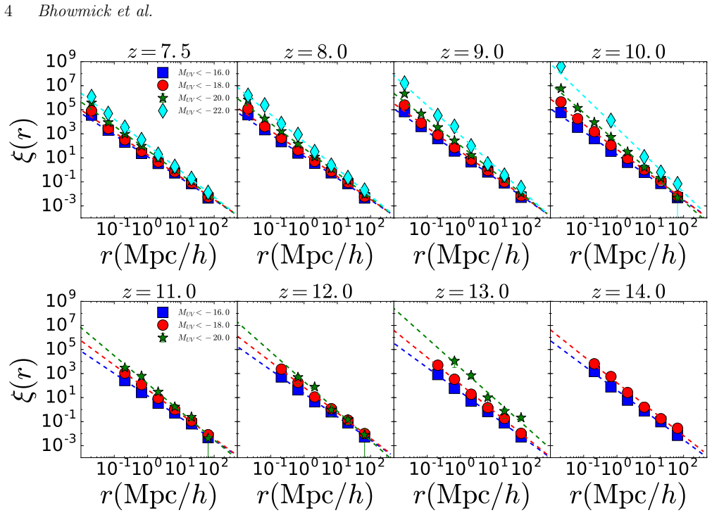
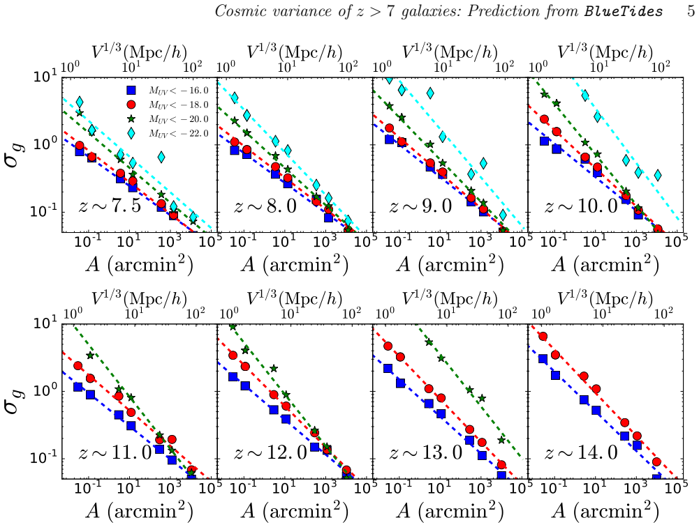
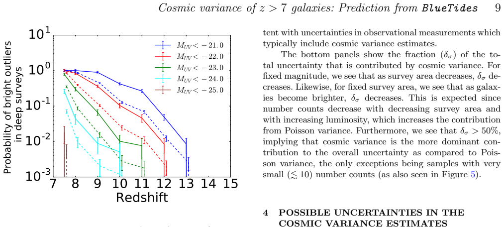
The load-bearing object is the cosmic variance statistic $\sigma_g^2 = (1/V^2)\int_V \int_V \xi_{gg}(r_1,r_2)\,d^3r_1\,d^3r_2$, where $\xi_{gg}$ is the two-point galaxy correlation function; it measures the excess field-to-field scatter in counts beyond Poisson noise. BlueTides supplies $\xi_{gg}$ for a UV-magnitude-limited galaxy population, and the paper condenses it into power-law fits $\xi(r)=(r/r_0)^\gamma$ and $\sigma_g=\Sigma A^\beta$, with a universal redshift-width scaling $(\Delta z/\Delta z_{\rm ref})^{-0.32}$. For small surveys (JWST medium/deep and lensed fields), the paper also counts galaxies in many simulated sub-volumes to obtain the full probability distribution of overdensities, which yields rare-outlier detection probabilities.
What would settle it
Compare the observed number-count scatter across many independent JWST fields, for example repeated $100\,\mathrm{arcmin}^2$ pointings at fixed $M_{\rm UV}<-16$ and $z\approx9$–$11$; the sample variance of those counts should equal the predicted $\sigma_g\approx20$–$50\%$, and a measured scatter outside this range after accounting for selection effects would falsify the BlueTides bias.
Extended reading notes
Core claim
The central claim is that for $z>7$ galaxies, cosmic variance is substantial and is the dominant component of the total uncertainty in every planned survey except those with fewer than about ten expected galaxies. Specifically, the paper predicts $\sigma_g\sim3\text{--}10\%$ for WFIRST's $10\,\mathrm{deg}^2$ field, $\sigma_g\sim20\text{--}50\%$ for JWST medium/deep surveys up to $A\sim100\,\mathrm{arcmin}^2$, and $\sigma_g\gtrsim40\%$ for lensed surveys; to keep the variance below $100\%$, effective volumes of $\gtrsim(8\,\mathrm{Mpc}/h)^3$ at $z\sim12$ and $\gtrsim(12\,\mathrm{Mpc}/h)^3$ at $z\sim14$ are required. The authors obtain these numbers from BlueTides, a $(400\,\mathrm{Mpc}/h)^3$ hydrodynamic simulation, by integrating the simulated two-point correlation function over mock survey volumes and, for small volumes, by building the full distribution of number counts across thousands of realizations.
Load-bearing premise
The simulation's mapping between galaxy UV brightness and dark-matter halo mass—and hence the clustering bias of $M_{\rm UV}$-limited samples—matches the real universe at $z=7.5$–$14$; if that mapping is wrong, every predicted cosmic variance shifts.
Editorial extensions
If this is right
- JWST's JADES-medium/deep and CEERS surveys should expect 20–50% field-to-field scatter in $M_{\rm UV}<-16$ to $-20$ samples at $z\sim7.5$–$11$; for example, roughly $2200\pm450$ galaxies at $z\sim7.5$ in a $100\,\mathrm{arcmin}^2$ field.
- WFIRST's $10\,\mathrm{deg}^2$ survey keeps cosmic variance at 3–10% for most samples, making it the cleanest platform for luminosity-function shape measurements at $z>7$.
- Lensed surveys probing the faint end have $\sigma_g\gtrsim40\%$, so their luminosity-function constraints are meaningful only if effective volumes exceed roughly $(8\text{--}12\,\mathrm{Mpc}/h)^3$, depending on redshift.
- Cosmic variance rather than Poisson noise sets the error budget for essentially all upcoming surveys; published luminosity functions at $z>7$ should carry cosmic-variance terms or risk overstating constraints.
Reading between the lines
- If the simulation's galaxy–halo connection is representative, the predicted scatter can be tested directly: the field-to-field dispersion in number counts across independent JWST fields should match $\sigma_g$, and a mismatch would localize where the galaxy–halo connection fails.
- The shallow power-law scaling $\sigma_g\propto A^{-0.25\ldots-0.45}$ means that enlarging a single field is an inefficient cure; several well-separated medium fields would reduce cosmic variance more effectively than one deep pencil beam.
- Because BlueTides contains no regions underdense by more than $2\sigma$, the predicted distribution of overdensities is asymmetric; survey teams can use this to decide whether a claimed 'void' field is physically plausible.
- The same machinery could be extended to stellar-mass-selected samples or to $z\sim6$–$7$ if the simulation's clustering is recalibrated, making the estimator useful beyond UV luminosity functions.
Signed reviews
Editorial analysis
A structured set of objections, weighed in public.
Referee Report
Summary. The paper uses the BlueTides cosmological hydrodynamic simulation (400 Mpc/h box, WMAP9 cosmology) to estimate the cosmic variance of z>7 galaxies selected by rest-frame UV absolute magnitude thresholds M_UV ~ -16 to -22, over survey areas from ~0.1 arcmin^2 to 10 deg^2 and redshifts 7.5-14. The authors fit the simulated two-point correlation function with power laws, integrate it over model survey volumes to obtain sigma_g, validate against subvolume number-count distributions for small/medium fields, and package the results as fitting functions and a public online calculator. They apply the estimator to JWST medium/deep surveys, WFIRST 1 and 10 deg^2 fields, and lensed surveys, concluding that cosmic variance ranges from a few percent for large WFIRST fields to tens of percent for JWST fields and >=40% for lensed surveys, and that cosmic variance generally dominates the Poisson uncertainty for samples with more than about 10 galaxies.
Significance. If the underlying BlueTides galaxy-halo connection is representative, these are useful, directly usable predictions for interpreting and planning high-redshift surveys. The paper's strengths are the large simulation volume, the transparent pipeline from correlation function to sigma_g, the explicit fitting functions and public calculator, and the internal cross-check between the correlation-integral method and the subvolume number-count method. The main scientific conclusions are however currently overstated in two ways: the claim that cosmic variance dominates Poisson variance 'in all current and upcoming surveys' is contradicted by the paper's own Table 2, and the quantitative predictions are presented without an uncertainty budget despite acknowledged shot-noise and modeling limitations.
major comments (3)
- [Abstract; Section 5; Table 2] The claim that cosmic variance is larger than Poisson variance except for samples with N ≲ 10 is internally contradicted by Table 2. In the 10 deg^2 rows, z=11, M_UV<-20 has ⟨N⟩=168 with δN_cosmic=7 and δN_poisson=13, and z=14, M_UV<-18 has ⟨N⟩=102 with δN_cosmic=4 and δN_poisson=10; in both cases N>10 and the Poisson uncertainty exceeds the cosmic-variance uncertainty. The 1 deg^2 row at z=14, M_UV<-18 likewise has N=10.6 with δN_cosmic=2.1 and δN_poisson=3.3. These rows make the abstract sentence 'cosmic variance is larger than Poisson variance and forms the dominant component of the overall uncertainty in all current and upcoming surveys' false as written, and they also conflict with Section 5's statement that cosmic variance dominates except for bins with ≲10 objects. The authors should either restrict the dominance claim to the small-area/JWST-like geometries shown in Figure 5 or provide a corrected quantitative condition (e.g., involving both N and the amplitude of sigma_g); the 10 deg^2 WFIRST-like points should be added to Figure 5.
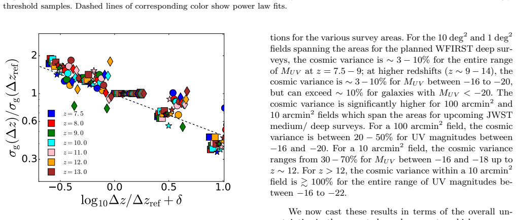
- [§3.2.2, Eq. (5); §3.4] The redshift-bin-width scaling sigma_g(Δz)/sigma_g(Δz_ref) = (Δz/Δz_ref)^{-0.32} is presented as universal, but the supporting Figure 3 shows only M_UV<-16 galaxies. The calculator CV_AT_COSMIC_DAWN then applies this exponent to every M_UV threshold and redshift in Table 1 via interpolation (§3.4). If the exponent depends on magnitude or redshift at z>7, the public estimates will be biased outside the single tested case. Please show the Δz dependence for at least a bright sample (e.g., M_UV<-20) and for a higher-redshift snapshot, or restrict Eq. (5) with appropriate caveats.
- [§3.1, Table 1; §4] The quantitative predictions are presented without an uncertainty budget. Table 1 lists power-law parameters r0 and gamma (and the derived Sigma, beta) with no error bars, and Figures 2 and 4 show no uncertainties on sigma_g; Section 4 provides only a qualitative discussion of systematic differences (e.g., 25-30% from cosmology) and does not propagate these or the fitting errors into the quoted values. This matters most at the bright end: Section 3.3.1 states that M_UV<-22 clustering 'could not be accurately probed due to excessive shot noise,' yet Table 1 still reports fits for M_UV=-22 at z=7.5-12 and the text quotes >10% cosmic variance for M_UV<-20 at z>10. Please provide uncertainties on the fitted parameters and sigma_g values, or explicitly flag the affected regimes as upper/lower limits.
minor comments (5)
- [§3.2.1, Eq. (4)] Equation (4) defines the power law with exponent beta, but the text states 'where α is the power-law exponent'; the symbol should be beta.
- [Table 1] At z=9, M_UV=-18, the fitted value gamma=-2.98 is likely a typo and breaks the monotonic trend with luminosity and redshift; please check and correct.
- [Figure 3 caption] The caption states that squares correspond to a survey area of 10 arcsec^2, which is inconsistent with the stated range of BlueTides validity (~0.1 arcmin^2 and above); this should likely be 10 arcmin^2.
- [Table 2 caption] Please state explicitly that deltaN_cosmic and deltaN_poisson are 1-sigma uncertainties, and clarify whether they are computed from the correlation-function integral or from the subvolume distribution, since both estimators are used in the paper.
- [References] The reference 'McCracken, H. J. et al., 2012' is formatted inconsistently with the other author-year references; it should be formatted in the same style.
Circularity Check
Cosmic variance is computed from simulated correlation functions via the standard volume integral; the fitting functions are data compressions, not fitted to the predicted variances, so no circularity.
full rationale
The central quantity sigma_g is obtained by Eq. (2) as an integral of the simulated two-point correlation function xi_gg over the survey volume, following the standard Peebles (1980) relation. xi_gg is measured directly from BlueTides galaxies and is not defined in terms of sigma_g or survey number counts, so the derivation does not reduce to its own output by definition. The power-law fits in Table 1 and Eq. (4)-(5) are compressions of the simulated clustering and computed variances, not parameters fitted to the target observable. The paper also cross-checks the integral method against direct sub-volume number-count distributions in Section 3.3.1, providing an independent internal check. The galaxy bias entering the calculation is an external modeling assumption of BlueTides, and the paper explicitly acknowledges in Section 4 that different cosmology or galaxy-formation physics would change the estimates; this is a modeling uncertainty, not circularity. Self-citations to Bhowmick et al. (2018a,b) are prior simulation predictions with independent content and are not invoked as a uniqueness theorem forcing the present result. No step in the derivation is equivalent to its input by construction. A possible inconsistency between the paper's blanket statement that cosmic variance dominates Poisson variance and the numbers in Table 2 would be an internal quantitative issue, not a circularity.
Assumptions & free parameters
free parameters (3)
- r0 and gamma power-law fit to BlueTides xi(r) for each M_UV threshold and redshift =
See Table 1
- Sigma and beta power-law fit to sigma_g(A) for each M_UV threshold and redshift =
See Table 1
- Redshift bin width scaling exponent alpha =
-0.32
assumptions (9)
- domain assumption BlueTides simulation with WMAP9 cosmology and its subgrid star formation, feedback, and reionization models produces realistic z>7 galaxies.
- domain assumption The galaxy SEDs computed with PEGASE-v2 and a Chabrier IMF give accurate rest-frame M_UV magnitudes.
- domain assumption Dust extinction is negligible for M_UV-limited samples with M_UV > -22.
- domain assumption The two-point correlation function of BlueTides galaxies is well-described by a single power law on all scales contributing to the cosmic variance integral.
- domain assumption Survey volumes can be approximated as cuboids with fixed transverse extent and no redshift evolution across the bin.
- domain assumption Subvolumes extracted from the periodic simulation box are independent realizations of the survey field.
- domain assumption The lensed-survey effective volumes from Livermore et al. (2017) are correct.
- domain assumption Linear interpolation between tabulated M_UV and redshift entries is sufficiently accurate for the calculator.
- standard math Standard cosmological and mathematical tools, including the Peebles (1980) integral formula and Poisson counting statistics, apply.
Cite this review
Pith. "Pith review of Cosmic variance of $z>7$ galaxies: Prediction from BlueTides." pith.science (2026). https://pith.science/paper/PNYW3WMD
@misc{pith2026190802787,
  author       = {Pith},
  title        = {Pith review of: Cosmic variance of $z>7$ galaxies: Prediction from BlueTides},
  year         = {2026},
  howpublished = {\url{https://pith.science/paper/PNYW3WMD}},
  note         = {Machine review of arXiv:1908.02787}
}
abstract
In the coming decade, a new generation of telescopes, including JWST and WFIRST, will probe the period of the formation of first galaxies and quasars, and open up the last frontier for structure formation. Recent simulations as well as observations have suggested that these galaxies are strongly clustered (with large scale bias $\gtrsim6$), and therefore have significant cosmic variance. In this work, we use \texttt{BlueTides}, the largest volume cosmological simulation of galaxy formation, to directly estimate the cosmic variance for current and upcoming surveys. Given its resolution and volume, \texttt{BlueTides} can probe the bias and cosmic variance of $z>7$ galaxies between magnitude $M_{UV}\sim-16$ to $M_{UV}\sim-22$ over survey areas $\sim0.1\ \mathrm{arcmin}^2$ to $\sim 10~\mathrm{deg}^2$. Within this regime, the cosmic variance decreases with survey area/ volume as a power law with exponents between $\sim-0.25$ to $\sim-0.45$. For the planned $10~\mathrm{deg}^2$ field of WFIRST, the cosmic variance is between $3\%$ to $10\%$. Upcoming JWST medium/ deep surveys with areas up to $A\sim100\ \mathrm{arcmin}^2$ will have cosmic variance ranging from $\sim 20-50\%$. Lensed surveys have the highest cosmic variance $\gtrsim 40\%$; the cosmic variance of $M_{UV}\lesssim-16$ galaxies is $\lesssim100\%$ up to $z\sim11$. At higher redshifts such as $z\sim12~(14)$, effective volumes of $\gtrsim(8~\mathrm{Mpc}/h)^3$ ($\gtrsim(12\ \mathrm{Mpc}/h)^3$) are required to limit the cosmic variance to within $100\%$. Finally, we find that cosmic variance is larger than Poisson variance and forms the dominant component of the overall uncertainty in all current and upcoming surveys. We present our calculations in the form of simple fitting functions and an online cosmic variance calculator (CV_AT_COSMIC_DAWN) which we publicly release.
Figures
Figures from the paper (7 more)




Reference graph
Works this paper leans on
-
[1]
Artale M. C., et al., 2017, @doi [ ] 10.1093/mnras/stx1263 , https://ui.adsabs.harvard.edu/abs/2017MNRAS.470.1771A 470, 1771
-
[2]
Ba \ n ados E., et al., 2018, @doi [ ] 10.1038/nature25180 , http://adsabs.harvard.edu/abs/2018Natur.553..473B 553, 473
-
[3]
Barone-Nugent R. L., et al., 2014, @doi [ ] 10.1088/0004-637X/793/1/17 , http://adsabs.harvard.edu/abs/2014ApJ...793...17B 793, 17
-
[4]
Battaglia N., Trac H., Cen R., Loeb A., 2013, @doi [ ] 10.1088/0004-637X/776/2/81 , http://adsabs.harvard.edu/abs/2013ApJ...776...81B 776, 81
-
[5]
Behroozi P. S., Wechsler R. H., Wu H.-Y., 2013, @doi [ ] 10.1088/0004-637X/762/2/109 , http://adsabs.harvard.edu/abs/2013ApJ...762..109B 762, 109
-
[6]
Bhowmick A. K., Di Matteo T., Feng Y., Lanusse F., 2018a, @doi [ ] 10.1093/mnras/stx3149 , https://ui.adsabs.harvard.edu/\#abs/2018MNRAS.474.5393B 474, 5393
-
[7]
Bhowmick A. K., Campbell D., Di Matteo T., Feng Y., 2018b, @doi [ ] 10.1093/mnras/sty2128 , https://ui.adsabs.harvard.edu/\#abs/2018MNRAS.480.3177B 480, 3177
-
[8]
Blaizot J., et al., 2006, @doi [ ] 10.1111/j.1365-2966.2006.10367.x , https://ui.adsabs.harvard.edu/abs/2006MNRAS.369.1009B 369, 1009
arXiv 2006
Show all 74 references
-
[9]
J., et al., 2015, @doi [ ] 10.1088/0004-637X/803/1/34 , https://ui.adsabs.harvard.edu/abs/2015ApJ...803...34B 803, 34
Bouwens R. J., et al., 2015, @doi [ ] 10.1088/0004-637X/803/1/34 , https://ui.adsabs.harvard.edu/abs/2015ApJ...803...34B 803, 34
2015 doi
-
[10]
J., Oesch P
Bouwens R. J., Oesch P. A., Illingworth G. D., Ellis R. S., Stefanon M., 2017, @doi [ ] 10.3847/1538-4357/aa70a4 , https://ui.adsabs.harvard.edu/\#abs/2017ApJ...843..129B 843, 129
2017 doi
-
[11]
Brada c M., et al., 2009, @doi [The Astrophysical Journal] 10.1088/0004-637x/706/2/1201 , 706, 1201
2009 doi
-
[12]
C., Padmanabhan N., Mao Y.-Y., Zentner A
Campbell D., van den Bosch F. C., Padmanabhan N., Mao Y.-Y., Zentner A. R., Lange J. U., Jiang F., Villarreal A., 2018, @doi [ ] 10.1093/mnras/sty495 , https://ui.adsabs.harvard.edu/abs/2018MNRAS.477..359C 477, 359
2018 doi
-
[13]
Chabrier G., 2003, @doi [ ] 10.1086/376392 , http://adsabs.harvard.edu/abs/2003PASP..115..763C 115, 763
2003 doi
-
[14]
J., Li C., Wang H., Yang X., Zhou S., Zhang Y., 2019, @doi [ ] 10.3847/1538-4357/ab0208 , https://ui.adsabs.harvard.edu/abs/2019ApJ...872..180C 872, 180
Chen Y., Mo H. J., Li C., Wang H., Yang X., Zhou S., Zhang Y., 2019, @doi [ ] 10.3847/1538-4357/ab0208 , https://ui.adsabs.harvard.edu/abs/2019ApJ...872..180C 872, 180
2019 doi
-
[15]
S., White S
Davis M., Efstathiou G., Frenk C. S., White S. D. M., 1985, @doi [ ] 10.1086/163168 , http://adsabs.harvard.edu/abs/1985ApJ...292..371D 292, 371
1985 doi
-
[16]
Di Matteo T., Springel V., Hernquist L., 2005, @doi [ ] 10.1038/nature03335 , http://adsabs.harvard.edu/abs/2005Natur.433..604D 433, 604
2005 doi
-
[17]
Di Matteo T., Croft R. A. C., Feng Y., Waters D., Wilkins S., 2017, @doi [ ] 10.1093/mnras/stx319 , http://adsabs.harvard.edu/abs/2017MNRAS.467.4243D 467, 4243
2017 doi
-
[18]
Duncan K., et al., 2014, @doi [ ] 10.1093/mnras/stu1622 , http://adsabs.harvard.edu/abs/2014MNRAS.444.2960D 444, 2960
2014 doi
-
[19]
Feng Y., Di Matteo T., Croft R., Tenneti A., Bird S., Battaglia N., Wilkins S., 2015, @doi [ ] 10.1088/2041-8205/808/1/L17 , http://adsabs.harvard.edu/abs/2015ApJ...808L..17F 808, L17
2015 doi
-
[20]
A., Bird S., Battaglia N., Wilkins S., 2016, @doi [ ] 10.1093/mnras/stv2484 , http://adsabs.harvard.edu/abs/2016MNRAS.455.2778F 455, 2778
Feng Y., Di-Matteo T., Croft R. A., Bird S., Battaglia N., Wilkins S., 2016, @doi [ ] 10.1093/mnras/stv2484 , http://adsabs.harvard.edu/abs/2016MNRAS.455.2778F 455, 2778
2016 doi
-
[21]
Cycle 0 Early Release Science
Finkelstein S., et al., 2017, The Cosmic Evolution Early Release Science (CEERS) Survey , JWST Proposal ID 1345. Cycle 0 Early Release Science
2017
-
[22]
Fioc M., Rocca-Volmerange B., 1997, , http://adsabs.harvard.edu/abs/1997A
1997
-
[23]
P., et al., 2006, @doi [ ] 10.1007/s11214-006-8315-7 , https://ui.adsabs.harvard.edu/\#abs/2006SSRv..123..485G 123, 485
Gardner J. P., et al., 2006, @doi [ ] 10.1007/s11214-006-8315-7 , https://ui.adsabs.harvard.edu/\#abs/2006SSRv..123..485G 123, 485
2006 doi
-
[24]
A., et al., 2011, @doi [ ] 10.1088/0067-0049/197/2/35 , https://ui.adsabs.harvard.edu/abs/2011ApJS..197...35G 197, 35
Grogin N. A., et al., 2011, @doi [ ] 10.1088/0067-0049/197/2/35 , https://ui.adsabs.harvard.edu/abs/2011ApJS..197...35G 197, 35
2011 doi
-
[25]
Harikane Y., et al., 2016, @doi [ ] 10.3847/0004-637X/821/2/123 , http://adsabs.harvard.edu/abs/2016ApJ...821..123H 821, 123
2016 doi
-
[26]
Hinshaw G., et al., 2013, @doi [ ] 10.1088/0067-0049/208/2/19 , http://adsabs.harvard.edu/abs/2013ApJS..208...19H 208, 19
2013 doi
-
[27]
Ishigaki M., Kawamata R., Ouchi M., Oguri M., Shimasaku K., Ono Y., 2018, @doi [ ] 10.3847/1538-4357/aaa544 , https://ui.adsabs.harvard.edu/abs/2018ApJ...854...73I 854, 73
2018 doi
-
[28]
Jauzac M., et al., 2015, @doi [ ] 10.1093/mnras/stv1402 , https://ui.adsabs.harvard.edu/abs/2015MNRAS.452.1437J 452, 1437
2015 doi
-
[29]
Kashikawa N., et al., 2004, @doi [ ] 10.1093/pasj/56.6.1011 , https://ui.adsabs.harvard.edu/abs/2004PASJ...56.1011K 56, 1011
2004 doi
-
[30]
H., Hernquist L., 1996, @doi [ ] 10.1086/192305 , http://adsabs.harvard.edu/abs/1996ApJS..105...19K 105, 19
Katz N., Weinberg D. H., Hernquist L., 1996, @doi [ ] 10.1086/192305 , http://adsabs.harvard.edu/abs/1996ApJS..105...19K 105, 19
1996 doi
-
[31]
Kawamata R., Oguri M., Ishigaki M., Shimasaku K., Ouchi M., 2016, @doi [ ] 10.3847/0004-637X/819/2/114 , http://adsabs.harvard.edu/abs/2016ApJ...819..114K 819, 114
2016 doi
-
[32]
Khandai N., Di Matteo T., Croft R., Wilkins S., Feng Y., Tucker E., DeGraf C., Liu M.-S., 2015, @doi [ ] 10.1093/mnras/stv627 , https://ui.adsabs.harvard.edu/abs/2015MNRAS.450.1349K 450, 1349
2015 doi
-
[33]
M., et al., 2017, in American Astronomical Society Meeting Abstracts \#230
Koekemoer A. M., et al., 2017, in American Astronomical Society Meeting Abstracts \#230. p. 316.13
2017
-
[34]
R., Gnedin N
Krumholz M. R., Gnedin N. Y., 2011, @doi [ ] 10.1088/0004-637X/729/1/36 , http://adsabs.harvard.edu/abs/2011ApJ...729...36K 729, 36
2011 doi
-
[35]
Laporte N., et al., 2012, @doi [ ] 10.1051/0004-6361/201219486 , https://ui.adsabs.harvard.edu/abs/2012A&A...542L..31L 542, L31
2012 doi
-
[36]
C., Finkelstein S
Livermore R. C., Finkelstein S. L., Lotz J. M., 2017, @doi [ ] 10.3847/1538-4357/835/2/113 , http://adsabs.harvard.edu/abs/2017ApJ...835..113L 835, 113
2017 doi
-
[37]
McCracken, H. J. et al., 2012, @doi [A&A] 10.1051/0004-6361/201219507 , 544, A156
2012 doi
-
[38]
J., McLure R
McLeod D. J., McLure R. J., Dunlop J. S., 2016, @doi [ ] 10.1093/mnras/stw904 , https://ui.adsabs.harvard.edu/abs/2016MNRAS.459.3812M 459, 3812
2016 doi
-
[39]
G., Castellano M., Grazian A., 2016, @doi [ ] 10.3847/0004-637X/818/1/90 , https://ui.adsabs.harvard.edu/abs/2016ApJ...818...90M 818, 90
Menci N., Sanchez N. G., Castellano M., Grazian A., 2016, @doi [ ] 10.3847/0004-637X/818/1/90 , https://ui.adsabs.harvard.edu/abs/2016ApJ...818...90M 818, 90
2016 doi
-
[40]
G., 2017, @doi [ ] 10.3847/1538-4357/836/1/61 , https://ui.adsabs.harvard.edu/abs/2017ApJ...836...61M 836, 61
Menci N., Merle A., Totzauer M., Schneider A., Grazian A., Castellano M., Sanchez N. G., 2017, @doi [ ] 10.3847/1538-4357/836/1/61 , https://ui.adsabs.harvard.edu/abs/2017ApJ...836...61M 836, 61
2017 doi
-
[41]
P., Somerville R
Moster B. P., Somerville R. S., Maulbetsch C., van den Bosch F. C., Macci \`o A. V., Naab T., Oser L., 2010, @doi [ ] 10.1088/0004-637X/710/2/903 , https://ui.adsabs.harvard.edu/\#abs/2010ApJ...710..903M 710, 903
2010 doi
-
[42]
P., Somerville R
Moster B. P., Somerville R. S., Newman J. A., Rix H.-W., 2011, @doi [ ] 10.1088/0004-637X/731/2/113 , https://ui.adsabs.harvard.edu/\#abs/2011ApJ...731..113M 731, 113
2011 doi
-
[43]
Nelson D., et al., 2015, @doi [Astronomy and Computing] https://doi.org/10.1016/j.ascom.2015.09.003 , 13, 12
2015 doi
-
[44]
Ni Y., Di Matteo T., Feng Y., Croft R. A. C., Tenneti A., 2018, @doi [ ] 10.1093/mnras/sty2616 , https://ui.adsabs.harvard.edu/\#abs/2018MNRAS.481.4877N 481, 4877
2018 doi
-
[45]
arXiv:1904.01604
Ni Y., Wang M.-Y., Feng Y., Di Matteo T., 2019, arXiv e-prints, https://ui.adsabs.harvard.edu/abs/2019arXiv190401604N p. arXiv:1904.01604
2019 arXiv
-
[46]
A., et al., 2016, @doi [ ] 10.3847/0004-637X/819/2/129 , https://ui.adsabs.harvard.edu/abs/2016ApJ...819..129O 819, 129
Oesch P. A., et al., 2016, @doi [ ] 10.3847/0004-637X/819/2/129 , https://ui.adsabs.harvard.edu/abs/2016ApJ...819..129O 819, 129
2016 doi
-
[47]
A., et al., 2018, @doi [ ] 10.3847/1538-4365/aacb30 , https://ui.adsabs.harvard.edu/abs/2018ApJS..237...12O 237, 12
Oesch P. A., et al., 2018, @doi [ ] 10.3847/1538-4365/aacb30 , https://ui.adsabs.harvard.edu/abs/2018ApJS..237...12O 237, 12
2018 doi
-
[48]
Park J., et al., 2017, @doi [ ] 10.1093/mnras/stx1884 , https://ui.adsabs.harvard.edu/\#abs/2017MNRAS.472.1995P 472, 1995
2017 doi
-
[49]
Peebles P. J. E., 1980, The large-scale structure of the universe
1980
-
[50]
Planck Collaboration et al., 2016, @doi [ ] 10.1051/0004-6361/201525830 , https://ui.adsabs.harvard.edu/abs/2016A&A...594A..13P 594, A13
2016 doi
-
[51]
Rafelski M., et al., 2015, @doi [ ] 10.1088/0004-6256/150/1/31 , https://ui.adsabs.harvard.edu/abs/2015AJ....150...31R 150, 31
2015 doi
-
[52]
Schaye J., et al., 2015, @doi [ ] 10.1093/mnras/stu2058 , https://ui.adsabs.harvard.edu/abs/2015MNRAS.446..521S 446, 521
2015 doi
-
[53]
S., Dav \'e R., 2015, @doi [ ] 10.1146/annurev-astro-082812-140951 , https://ui.adsabs.harvard.edu/abs/2015ARA&A..53...51S 53, 51
Somerville R. S., Dav \'e R., 2015, @doi [ ] 10.1146/annurev-astro-082812-140951 , https://ui.adsabs.harvard.edu/abs/2015ARA&A..53...51S 53, 51
2015 doi
-
[54]
S., Lee K., Ferguson H
Somerville R. S., Lee K., Ferguson H. C., Gardner J. P., Moustakas L. A., Giavalisco M., 2004, @doi [ ] 10.1086/378628 , https://ui.adsabs.harvard.edu/abs/2004ApJ...600L.171S 600, L171
2004 doi
-
[55]
S., Hopkins P
Somerville R. S., Hopkins P. F., Cox T. J., Robertson B. E., Hernquist L., 2008, @doi [ ] 10.1111/j.1365-2966.2008.13805.x , https://ui.adsabs.harvard.edu/abs/2008MNRAS.391..481S 391, 481
2008
-
[56]
Song M., et al., 2016, @doi [ ] 10.3847/0004-637X/825/1/5 , http://adsabs.harvard.edu/abs/2016ApJ...825....5S 825, 5
2016 doi
-
[57]
arXiv:1503.03757
Spergel D., et al., 2015, arXiv e-prints, https://ui.adsabs.harvard.edu/\#abs/2015arXiv150303757S p. arXiv:1503.03757
2015 arXiv
-
[58]
Springel V., Hernquist L., 2003, @doi [ ] 10.1046/j.1365-8711.2003.06206.x , http://adsabs.harvard.edu/abs/2003MNRAS.339..289S 339, 289
2003
-
[59]
Springel V., Di Matteo T., Hernquist L., 2005, @doi [ ] 10.1111/j.1365-2966.2005.09238.x , http://adsabs.harvard.edu/abs/2005MNRAS.361..776S 361, 776
2005
-
[60]
Tenneti A., Di Matteo T., Croft R., Garcia T., Feng Y., 2017, preprint, http://adsabs.harvard.edu/abs/2017arXiv170803373T ( @eprint arXiv 1708.03373 )
2017 arXiv
-
[61]
M., Di Matteo T., Croft R
Tenneti A., Wilkins S. M., Di Matteo T., Croft R. A. C., Feng Y., 2019, @doi [ ] 10.1093/mnras/sty3161 , https://ui.adsabs.harvard.edu/\#abs/2019MNRAS.483.1388T 483, 1388
2019 doi
-
[62]
L., Robertson B
Tinker J. L., Robertson B. E., Kravtsov A. V., Klypin A., Warren M. S., Yepes G., Gottl \"o ber S., 2010, @doi [ ] 10.1088/0004-637X/724/2/878 , http://adsabs.harvard.edu/abs/2010ApJ...724..878T 724, 878
2010 doi
-
[63]
Trenti M., Stiavelli M., 2008, @doi [ ] 10.1086/528674 , https://ui.adsabs.harvard.edu/abs/2008ApJ...676..767T 676, 767
2008 doi
-
[64]
arXiv:2004.11096
Ucci G., et al., 2020, arXiv e-prints, https://ui.adsabs.harvard.edu/abs/2020arXiv200411096U p. arXiv:2004.11096
2020 arXiv
-
[65]
Vogelsberger M., Genel S., Sijacki D., Torrey P., Springel V., Hernquist L., 2013, @doi [ ] 10.1093/mnras/stt1789 , http://adsabs.harvard.edu/abs/2013MNRAS.436.3031V 436, 3031
2013 doi
-
[66]
Vogelsberger M., et al., 2014, @doi [ ] 10.1093/mnras/stu1536 , http://adsabs.harvard.edu/abs/2014MNRAS.444.1518V 444, 1518
2014 doi
-
[67]
M., Di Matteo T., Feng Y., Croft R., Nagai D., 2016a, @doi [ ] 10.1093/mnrasl/slw100 , https://ui.adsabs.harvard.edu/abs/2016MNRAS.461L..51W 461, L51
Waters D., Wilkins S. M., Di Matteo T., Feng Y., Croft R., Nagai D., 2016a, @doi [ ] 10.1093/mnrasl/slw100 , https://ui.adsabs.harvard.edu/abs/2016MNRAS.461L..51W 461, L51
-
[68]
M., Croft R
Waters D., Di Matteo T., Feng Y., Wilkins S. M., Croft R. A. C., 2016b, @doi [ ] 10.1093/mnras/stw2000 , https://ui.adsabs.harvard.edu/abs/2016MNRAS.463.3520W 463, 3520
-
[69]
M., Feng Y., Di-Matteo T., Croft R., Stanway E
Wilkins S. M., Feng Y., Di-Matteo T., Croft R., Stanway E. R., Bouwens R. J., Thomas P., 2016a, @doi [ ] 10.1093/mnrasl/slw007 , http://adsabs.harvard.edu/abs/2016MNRAS.458L...6W 458, L6
-
[70]
M., Feng Y., Di-Matteo T., Croft R., Stanway E
Wilkins S. M., Feng Y., Di-Matteo T., Croft R., Stanway E. R., Bunker A., Waters D., Lovell C., 2016b, @doi [ ] 10.1093/mnras/stw1154 , http://adsabs.harvard.edu/abs/2016MNRAS.460.3170W 460, 3170
-
[71]
M., Feng Y., Di Matteo T., Croft R., Lovell C
Wilkins S. M., Feng Y., Di Matteo T., Croft R., Lovell C. C., Thomas P., 2018, @doi [ ] 10.1093/mnras/stx2588 , http://adsabs.harvard.edu/abs/2018MNRAS.473.5363W 473, 5363
2018 doi
-
[72]
J., van den Bosch F
Yang X., Mo H. J., van den Bosch F. C., Zhang Y., Han J., 2012, @doi [ ] 10.1088/0004-637X/752/1/41 , https://ui.adsabs.harvard.edu/abs/2012ApJ...752...41Y 752, 41
2012 doi
-
[73]
Yung L. Y. A., Somerville R. S., Popping G., Finkelstein S. L., Ferguson H. C., Dav \'e R., 2019a, arXiv e-prints, https://ui.adsabs.harvard.edu/abs/2019arXiv190105964Y p. arXiv:1901.05964
1901 arXiv
-
[74]
Yung L. Y. A., Somerville R. S., Finkelstein S. L., Popping G., Dav \'e R., 2019b, @doi [ ] 10.1093/mnras/sty3241 , https://ui.adsabs.harvard.edu/abs/2019MNRAS.483.2983Y 483, 2983
Reviewed August 14, 2026 · model on record in the stance chip above.
Discussion (0). Continue with ORCID to comment.