REVIEW 4 major objections 4 minor 42 references
A Bayesian Markov model with P\'olya-Gamma sampling for estimating individual behavior transition probabilities from accelerometer classifications
T0 review · 4 major / 4 minor · reviewed 2026-08-14 · deepseek-v4-flash
Pith's one-line read A Bayesian Markov model with Pólya-Gamma sampling estimates how habitat, time of day, and weather drive behavior transitions in accelerometer-classified geese.
desk verdict The ecological application is thoughtful, but the multinomial Pólya-Gamma sampler in Eq. (5) is invalid for four states, so the reported odds ratios likely do not correspond to the stated transition model. read the letter →
The pith
A machine-rendered reading of the paper's core claim, the machinery that carries it, and where it could break.
The reading
What carries the argument
The central object is a time-varying first-order Markov transition matrix $P_{nt}$ over four behaviors, with each row modeled by a multinomial logistic link, $\psi_{nijt}=\log(p_{nijt}/p_{niJt})=x_{nt}'\beta_{ij}$, where walking is the reference category. Two augmentations carry the argument: Pólya-Gamma latent variables, which turn the multinomial logistic likelihood into conditionally conjugate Gaussian updates for the coefficients $\beta_{ij}$, and multiple imputation, which draws $M=200$ behavior sequences from the random forest's classification probabilities $[S|A]$ and averages the Markov-model posterior over them. The machinery yields automatic Gibbs sampling without tuning and odds-ratio summaries for every covariate effect on each transition.
What would settle it
Take the video-verified training behaviors, fit the same Markov model once to the true labels and once to sequences imputed from the random forest for the same ACC fixes, and compare posterior transition coefficients; if the imputation-based estimates shift systematically away from the truth-labeled estimates, the assumed $[S|A]$ is miscalibrated and the reported habitat, weather, and diurnal effects are not trustworthy. A simpler version: recalibrate the random forest probabilities on a validation set and check whether any odds-ratio posterior moves by more than its credible interval.
Extended reading notes
Core claim
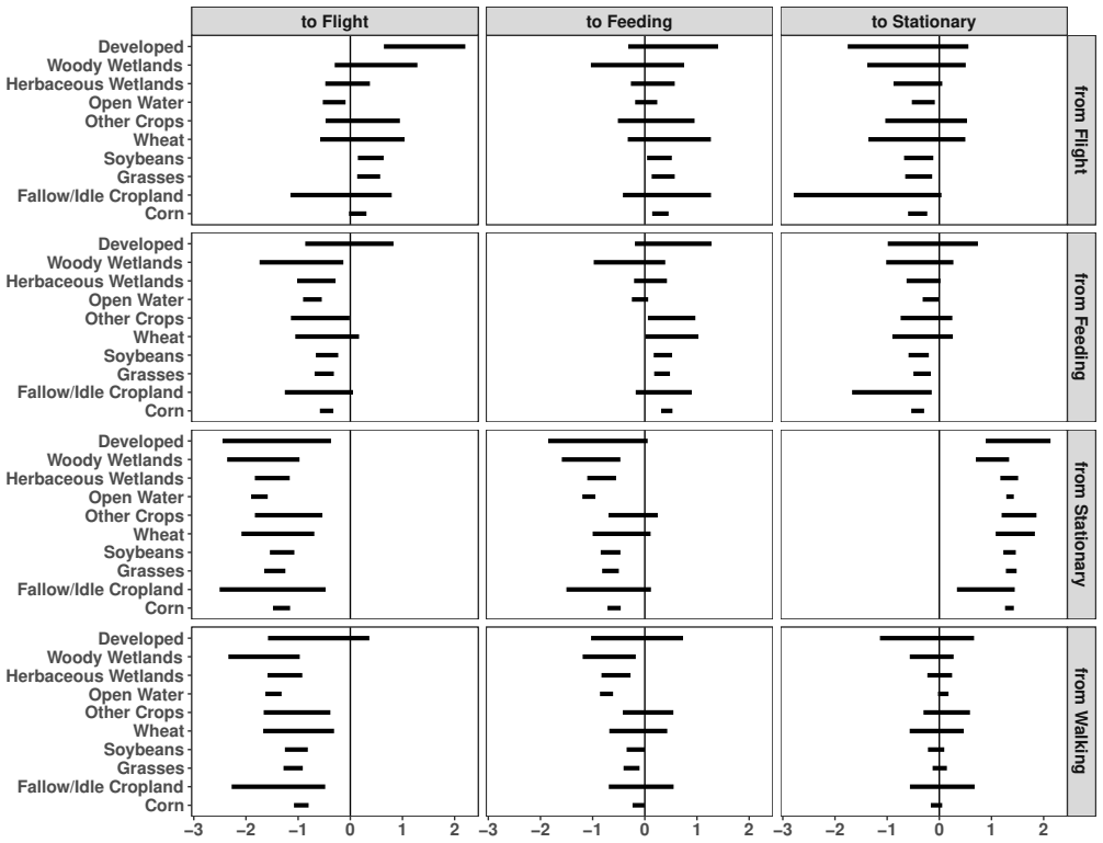
The central claim is that behavior transition probabilities can be estimated directly from classified accelerometer data with a first-order Markov model whose transition probabilities follow a multinomial logistic link, with Pólya-Gamma latent variables making posterior sampling automatic and with multiple imputation carrying the random forest classifier's uncertainty into the posterior. For six greater white-fronted geese in March 2018, the model finds significant habitat effects on nearly every transition probability, a strong diurnal cycle (increased stationary behavior at night, reduced flight and feeding), and weather effects concentrated on flight and feeding transitions, including opposing effects of daily minimum and maximum temperature on the probability of continuing to fly. The authors present the framework as a unifying way to use both acceleration and GPS data for behavioral inference.
Load-bearing premise
The load-bearing premise is that the random forest's predicted class probabilities give the true conditional distribution of behavior given the acceleration data, because behavior sequences imputed from those probabilities are then treated as the data for the Markov model; any miscalibration in the classifier flows directly into every transition estimate.
Editorial extensions
If this is right
- Habitat effects on behavior can be estimated without defining an availability distribution, so habitats used at similar rates can still be distinguished by the behaviors performed in them.
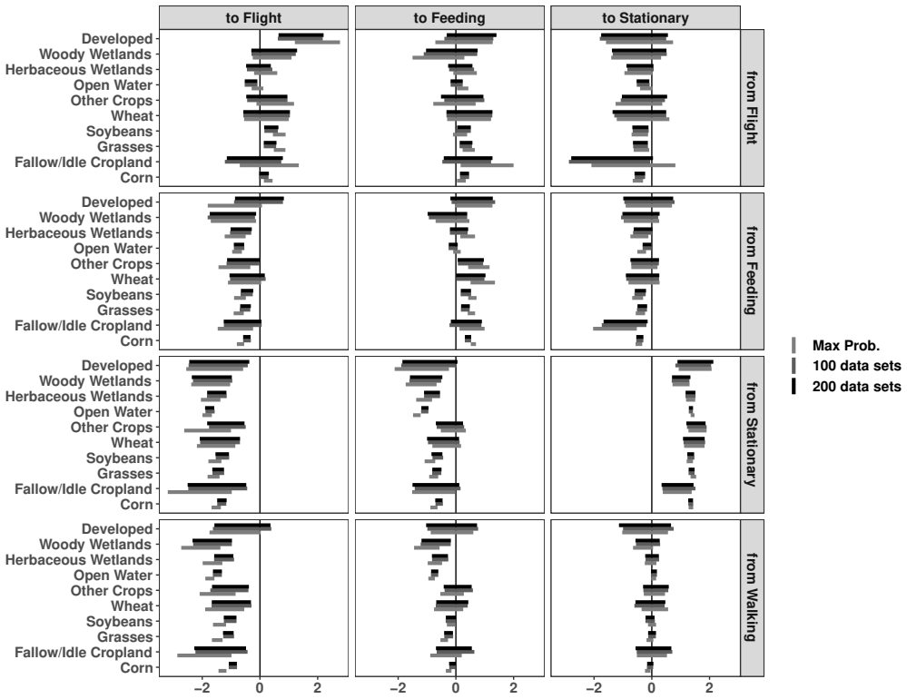
- Classification uncertainty is propagated: compared with using only the most likely behavior label, multiple imputation shrinks coefficient estimates toward zero and keeps credible intervals at least as wide.
- The Pólya-Gamma scheme removes the need to tune Metropolis-Hastings proposals for multinomial logistic transition models, making similar Bayesian behavior models easier to fit for other species.
- Transition-specific coefficients can expose asymmetric responses, such as weather changing the probability of remaining in flight but not the probability of leaving stationary behavior.
- Fitted transition matrices support posterior predictive simulation of behavior sequences, allowing comparisons of time allocation across habitats or weather scenarios.
Reading between the lines
- A natural extension the authors only gesture at is sharing coefficients across transitions for covariates like time of day, which appeared to act similarly across all from-states; a behavior-specific formulation would reduce parameter count and sharpen inference.
- Habitat and weather values are assigned to each ACC fix from the most recent GPS location, so a 30-minute GPS gap is mapped onto a 6-minute behavior scale; interpolating locations to ACC times would test whether the reported habitat effects are robust to this timing assumption.
- The sensitivity comparison suggests the direction of effects survives even using a single most-likely classification, implying the substantive conclusions may not hinge on the imputation count; a formal diagnostic for the number of imputations would strengthen the method.
- The paper notes the same augmentation can enter hidden Markov models; that route would let movement ecologists replace tuned HMM samplers with Pólya-Gamma updates when behavioral states are not directly observed.
Signed reviews
Editorial analysis
A structured set of objections, weighed in public.
Referee Report
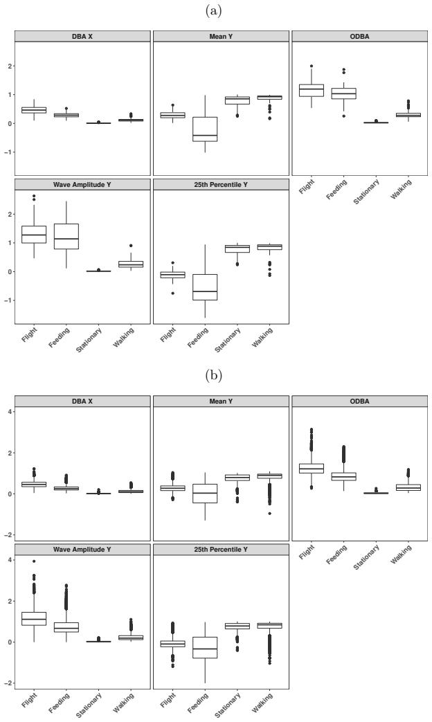
Summary. The paper proposes a two-stage Bayesian framework for inferring animal behavior transition probabilities from accelerometer (ACC) data. A random forest classifier assigns four behavior states (flying, feeding, stationary, walking) from ACC features, and multiple imputation (M = 200 imputed data sets) is used to propagate classification uncertainty. A first-order Markov model with multinomial logistic transition probabilities relates transitions to habitat, weather, and time-of-day covariates, with Pólya-Gamma latent variables used for Gibbs sampling of the coefficients. The method is applied to six greater white-fronted geese during March 2018, and the authors report significant habitat, diurnal, and weather effects on transition rates, with odds-ratio summaries and pairwise habitat comparisons.
Significance. If the methodology were correct, the paper would make a useful contribution to movement ecology: it explicitly models temporal dependence in behavior classifications, propagates classifier uncertainty via multiple imputation, and offers a computationally convenient Pólya-Gamma sampler for a nonhomogeneous Markov model. The full conditional distributions are provided, and the supplementary material includes sensitivity analyses for the number of imputations and posterior predictive checks. However, the central statistical claim is undermined by an incorrect likelihood representation in Eq. (5) and by full conditionals in the supplementary material that implement a different model. The ecological conclusions, while plausible and of interest, are currently not supported by the reported inference.
major comments (4)
- [Model Fitting, Eq. (5)] Equation (5) is not a valid algebraic representation of the multinomial logistic likelihood for J > 2. For a single transition with observed category j*, the right-hand product is logistic(η_{j*}) × Π_{j≠j*} (1 − logistic(η_j)). For J = 3 with reference category 3, this equals e^{ψ_{j*}}(e^{ψ_{j*}}+1)/D^2, where D = 1 + e^{ψ_1} + e^{ψ_2}; the extra factor (e^{ψ_{j*}}+1)/D depends on the parameters and on which category was observed, so the right side is not proportional to the multinomial probability e^{ψ_{j*}}/D. Consequently, the posterior sampled by the proposed algorithm is not the posterior of the multinomial logistic model in Eq. (2). Because every reported coefficient, odds ratio, and significance statement in Tables 1–2 and Figures 2–3 is produced by this sampler, the central inference of the paper is currently unsupported.
- [Supplementary Material S.3] The full conditionals in S.3 are exactly the updates for J−1 independent binary logistic regressions (one for each non-reference category), with response Y_ij and offset C_nijt. In a correct Pólya-Gamma sampler for the softmax likelihood, the update for β_ij must also account for the dependence of the other categories' offsets C_nik (k ≠ j) on β_ij; those terms are absent here. Thus the Markov chain targets the product-of-Bernoulli posterior rather than the multinomial logistic posterior. The reference to Theorem 1 of Polson et al. (2013) does not justify this multinomial construction; the authors need to use a valid multinomial Pólya-Gamma representation (for example, logistic-softmax or multivariate Pólya-Gamma) and rerun all analyses.
- [Multiple Imputation, Eq. (6)] Equation (6) assumes that the imputation distribution [S|A] is exactly the random forest classification probability, but no evidence is provided that these probabilities are calibrated, and the assumption that behavior labels are conditionally independent in time given ACC data is stated but not checked. If the random forest probabilities are miscalibrated or the classification errors are temporally correlated, the imputed behavior sequences are drawn from the wrong distribution and the bias propagates directly into all transition estimates. The sensitivity analysis in S.6 only varies the number of imputations, not the correctness of the imputation distribution, so it cannot address this concern. A calibration check on held-out ACC fixes, or an alternative imputation model with posterior predictive calibration, is needed.
- [Dataset] Habitat and weather covariates for each ACC fix are taken from the most recent GPS fix, with GPS at 30-minute intervals and ACC at 6-minute intervals (Dataset section). Last-observation-carried-forward can misassign habitat during flights or short stops, and no sensitivity analysis is reported for this choice. Since the paper's main ecological conclusions concern habitat-specific transition rates and weather effects, this measurement-error issue is load-bearing; at minimum, a comparison with interpolated locations or an analysis restricted to GPS-aligned fixes is required.
minor comments (4)
- [Equation (5) and S.3] The notation in the definition of C_nijt is garbled: the summation should be over k ≠ j, not over 'k, j'. Please correct the typesetting and make the notation consistent.
- [Results, Table 1] The text describing the corn coefficient as a 'mean effect' of 0.42 should say 'posterior mean of the log-odds coefficient' or 'log odds ratio', rather than 'mean effect', to avoid ambiguity.
- [Supplementary S.5 vs Results] The main text says the only transition without significant habitat differences was flight to stationary, while S.5 states that 'grazing to flight' was the only transition without significant pairwise differences. These statements should be reconciled, and the transit
- [Figure 4 caption] The caption says 'the upper triangular values and lower triangular values sum to 1'; this should clarify that corresponding row/column pairs (not the entire triangles) sum to 1.
Circularity Check
No circularity: imputed behaviors come from an external random forest; Markov coefficients are fitted outputs.
full rationale
The derivation chain is self-contained with respect to the ecological conclusions. The imputed behavior sequences used as data are drawn from [S|A], the random forest prediction distribution (Eq. 6: 'We assumed the distribution of the behavior labels given the ACC data, [S|A], is the prediction from the supervised classification random forest'), whose training labels came from video ground-truth (S.2), not from the Markov model. The Markov transition probabilities and covariate coefficients are then estimated from these imputed sequences; no ecological hypothesis or habitat/weather coefficient is fed back into the classifier or into the prior. Thus the claimed significant effects are outputs, not inputs. The Pólya-Gamma sampler is imported from external methodology (Polson et al. 2013; Holmes and Held 2006), and the only author-overlapping citation (Hooten et al. 2018, with Weegman) is motivational background, not load-bearing. The S.4 validation is an in-sample posterior predictive check against the same imputed data; it is therefore not an out-of-sample validation, but since the paper presents it as goodness-of-fit rather than as an independent prediction, this is a limitation, not circularity. The correctness concern about Eq. (5) (multinomial likelihood expressed as a product of binary logistic functions) is a misspecification issue, not circularity, because the alleged reduction is an error, not an equivalence-by-construction.
Assumptions & free parameters
free parameters (4)
- Prior variance fixed at 100 =
100
- Number of imputation data sets M =
200
- Random forest mtry =
4
- Habitat category aggregation =
10 categories
assumptions (4)
- domain assumption First-order Markov assumption: current behavior depends only on the immediately previous behavior.
- domain assumption The random forest predictive probabilities equal the true conditional distribution [S|A] of behavior given acceleration data.
- domain assumption Habitat and weather at each ACC fix are equal to the values at the most recent GPS fix, up to 30 minutes earlier.
- domain assumption Behavior labels are conditionally independent in time given ACC data.
Cite this review
Pith. "Pith review of A Bayesian Markov model with P\'olya-Gamma sampling for estimating individual behavior transition probabilities from accelerometer classifications." pith.science (2026). https://pith.science/paper/DOM75F2K
@misc{pith2026190802806,
  author       = {Pith},
  title        = {Pith review of: A Bayesian Markov model with P\'olya-Gamma sampling for estimating individual behavior transition probabilities from accelerometer classifications},
  year         = {2026},
  howpublished = {\url{https://pith.science/paper/DOM75F2K}},
  note         = {Machine review of arXiv:1908.02806}
}
read the original abstract
The use of accelerometers in wildlife tracking provides a fine-scale data source for understanding animal behavior and decision-making. Current methods in movement ecology focus on behavior as a driver of movement mechanisms. Our Markov model is a flexible and efficient method for inference related to effects on behavior that considers dependence between current and past behaviors. We applied this model to behavior data from six greater white-fronted geese (Anser albifrons frontalis) during spring migration in mid-continent North America and considered likely drivers of behavior, including habitat, weather and time of day effects. We modeled the transitions between flying, feeding, stationary and walking behavior states using a first-order Bayesian Markov model. We introduced P\'olya-Gamma latent variables for automatic sampling of the covariate coefficients from the posterior distribution and we calculated the odds ratios from the posterior samples. Our model provides a unifying framework for including both acceleration and Global Positioning System data. We found significant differences in behavioral transition rates among habitat types, diurnal behavior and behavioral changes due to weather. Our model provides straightforward inference of behavioral time allocation across used habitats, which is not amenable in activity budget or resource selection frameworks.
Figures


Figures from the paper (5 more)



Reference graph
Works this paper leans on
-
[1]
Albert, J. H. and Chib, S. (1993). ``Bayesian analysis of binary and polychotomous response data.''\ Journal of the American statistical Association , 88(422), 669--679
work page 1993
-
[2]
Altmann, J. (1974). ``Observational study of behavior: S ampling methods.''\ Behaviour , 49(3-4), 227--266
work page 1974
-
[3]
Baldassarre, G. A. (2014). Ducks, G eese, and S wans of N orth America , Vol. 1. JHU Press
work page 2014
-
[4]
Breed, M. D. and Moore, J. (2015). Animal B ehavior . Academic Press
work page 2015
-
[5]
Broekhuis, F., Gr \"u new \"a lder, S., McNutt, J. W., and Macdonald, D. W. (2014). ``Optimal hunting conditions drive circalunar behavior of a diurnal carnivore.''\ Behavioral Ecology , 25(5), 1268--1275
work page 2014
-
[6]
Brooks, S. P. and Gelman, A. (1998). ``General methods for monitoring convergence of iterative simulations.''\ Journal of computational and graphical statistics , 7(4), 434--455
work page 1998
-
[7]
Brown, J. H., Gillooly, J. F., Allen, A. P., Savage, V. M., and West, G. B. (2004). ``Toward a metabolic theory of ecology.''\ Ecology , 85(7), 1771--1789
work page 2004
-
[8]
Chakravarty, P., Cozzi, G., Ozgul, A., and Aminian, K. (2019). ``A novel biomechanical approach for animal behaviour recognition using accelerometers.''\ Methods in Ecology and Evolution
work page 2019
Show all 42 references
-
[9]
Chen, J., Zhu, J., Wang, Z., Zheng, X., and Zhang, B. (2013). ``Scalable inference for logistic-normal topic models.''\ Advances in Neural Information Processing Systems , 2445--2453
2013
-
[10]
Ely, C. R. (1992). ``Time allocation by G reater white-fronted geese: influence of diet, energy reserves and predation.''\ The Condor , 94(4), 857--870
1992
-
[11]
D., Glahder, C
Fox, A. D., Glahder, C. M., and Walsh, A. J. (2003). ``Spring migration routes and timing of G reenland white-fronted geese--results from satellite telemetry.''\ Oikos , 103(2), 415--425
2003
-
[12]
u hwirth-Schnatter, S. and Fr \
Fr \"u hwirth-Schnatter, S. and Fr \"u hwirth, R. (2007). ``Auxiliary mixture sampling with applications to logistic models.''\ Computational Statistics & Data Analysis , 51(7), 3509--3528
2007
-
[13]
u hwirth-Schnatter, S. and Fr \
Fr \"u hwirth-Schnatter, S. and Fr \"u hwirth, R. (2010). ``Data augmentation and MCMC for binary and multinomial logit models.''\ Statistical modelling and regression structures , Springer, 111--132
2010
-
[14]
Gelman, A., Hill, J., and Yajima, M. (2012). ``Why we (usually) don't have to worry about multiple comparisons.''\ Journal of Research on Educational Effectiveness , 5(2), 189--211
2012
-
[15]
R., Richardson, S., and Spiegelhalter, D
Gilks, W. R., Richardson, S., and Spiegelhalter, D. (1995). Markov chain Monte Carlo in practice . Chapman and Hall/CRC
1995
-
[16]
T., Howard, B., Banks, D
Glynn, C., Tokdar, S. T., Howard, B., Banks, D. L., et al.\@ (2019). ``Bayesian analysis of dynamic linear topic models.''\ Bayesian Analysis , 14(1), 53--80
2019
-
[17]
A., Blount, J
Harrison, X. A., Blount, J. D., Inger, R., Norris, D. R., and Bearhop, S. (2011). ``Carry-over effects as drivers of fitness differences in animals.''\ Journal of Animal Ecology , 80(1), 4--18
2011
-
[18]
R., et al.\@ (2014)
Heurich, M., Hilger, A., K \"u chenhoff, H., Andr \'e n, H., Bufka, L., Krofel, M., Mattisson, J., Odden, J., Persson, J., Rauset, G. R., et al.\@ (2014). ``Activity patterns of E urasian lynx are modulated by light regime and individual traits over a wide latitudinal range.''...
2014
-
[19]
Holmes, C. C. and Held, L. (2006). ``Bayesian auxiliary variable models for binary and multinomial regression.''\ Bayesian analysis , 1(1), 145--168
2006
-
[20]
M., Robertson, A
Holsclaw, T., Greene, A. M., Robertson, A. W., Smyth, P., et al.\@ (2017). ``Bayesian nonhomogeneous M arkov models via P \'o lya- G amma data augmentation with applications to rainfall modeling.''\ The Annals of Applied Statistics , 11(1), 393--426
2017
-
[21]
Hooten, M. B. and Hobbs, N. T. (2015). `` A guide to B ayesian model selection for ecologists.''\ Ecological Monographs , 85(1), 3--28
2015
-
[22]
B., Johnson, D
Hooten, M. B., Johnson, D. S., Hanks, E. M., and Lowry, J. H. (2010). ``Agent-based inference for animal movement and selection.''\ Journal of Agricultural, Biological and Environmental Statistics , 15(4), 523--538
2010
-
[23]
B., Johnson, D
Hooten, M. B., Johnson, D. S., McClintock, B. T., and Morales, J. M. (2017). Animal M ovement: S tatistical M odels for T elemetry D ata . CRC Press
2017
-
[24]
B., Scharf, H
Hooten, M. B., Scharf, H. R., Hefley, T. J., Pearse, A. T., and Weegman, M. D. (2018). ``Animal movement models for migratory individuals and groups.''\ Methods in Ecology and Evolution , 9(7), 1692--1705
2018
-
[25]
S., London, J
Johnson, D. S., London, J. M., Lea, M.-A., and Durban, J. W. (2008). ``Continuous-time correlated random walk model for animal telemetry data.''\ Ecology , 89(5), 1208--1215
2008
-
[26]
L., Reinecke, K
Krapu, G. L., Reinecke, K. J., Jorde, D. G., and Simpson, S. G. (1995). ``Spring-staging ecology of midcontinent greater white-fronted geese.''\ The Journal of wildlife management , 736--746
1995
-
[27]
A., Watanabe, Y
Leos-Barajas, V., Photopoulou, T., Langrock, R., Patterson, T. A., Watanabe, Y. Y., Murgatroyd, M., and Papastamatiou, Y. P. (2017). ``Analysis of animal accelerometer data using hidden M arkov models.''\ Methods in Ecology and Evolution , 8(2), 161--173
2017
-
[28]
Linderman, S., Johnson, M., and Adams, R. P. (2015). ``Dependent multinomial models made easy: S tick-breaking with the P \'o lya- G amma augmentation.''\ Advances in Neural Information Processing Systems , 3456--3464
2015
-
[29]
McClintock, B. T. (2017). ``Incorporating telemetry error into hidden M arkov models of animal movement using multiple imputation.''\ Journal of Agricultural, Biological and Environmental Statistics , 22(3), 249--269
2017
-
[30]
T., London, J
McClintock, B. T., London, J. M., Cameron, M. F., and Boveng, P. L. (2017). ``Bridging the gaps in animal movement: hidden behaviors and ecological relationships revealed by integrated data streams.''\ Ecosphere , 8(3), e01751
2017
-
[31]
and Blackwell, P
Michelot, T. and Blackwell, P. G. (2019). ``State-switching continuous-time correlated random walks.''\ Methods in Ecology and Evolution , 10(5), 637--649
2019
-
[32]
D., Photopoulou, T., and Patterson, T
Michelot, T., Langrock, R., Bestley, S., Jonsen, I. D., Photopoulou, T., and Patterson, T. A. (2017). ``Estimation and simulation of foraging trips in land-based marine predators.''\ Ecology , 98(7), 1932--1944
2017
-
[33]
M., Haydon, D
Morales, J. M., Haydon, D. T., Frair, J., Holsinger, K. E., and Fryxell, J. M. (2004). ``Extracting more out of relocation data: building movement models as mixtures of random walks.''\ Ecology , 85(9), 2436--2445
2004
-
[34]
Nathan, R., Spiegel, O., Fortmann-Roe, S., Harel, R., Wikelski, M., and Getz, W. M. (2012). ``Using tri-axial acceleration data to identify behavioral modes of free-ranging animals: general concepts and tools illustrated for griffon vultures.''\ Journal of Experimental Biology...
2012
-
[35]
A., Parton, A., Langrock, R., Blackwell, P
Patterson, T. A., Parton, A., Langrock, R., Blackwell, P. G., Thomas, L., and King, R. (2017). ``Statistical modelling of individual animal movement: an overview of key methods and a discussion of practical challenges.''\ AStA Advances in Statistical Analysis , 101(4), 399--438
2017
-
[36]
G., Scott, J
Polson, N. G., Scott, J. G., and Windle, J. (2013). ``Bayesian inference for logistic models using P \'o lya- G amma latent variables.''\ Journal of the American statistical Association , 108(504), 1339--1349
2013
-
[37]
S., Rotics, S., Harel, R., Spiegel, O., and Nathan, R
Resheff, Y. S., Rotics, S., Harel, R., Spiegel, O., and Nathan, R. (2014). ``Accele R ater: a web application for supervised learning of behavioral modes from acceleration measurements.''\ Movement Ecology , 2(1), 27
2014
-
[38]
Rubin, D. B. (2004). Multiple imputation for nonresponse in surveys , Vol. 81. John Wiley & Sons
2004
-
[39]
Rugg, D. J. and Buech, R. R. (1990). ``Analyzing time budgets with M arkov chains.''\ Biometrics , 1123--1131
1990
-
[40]
B., and Johnson, D
Scharf, H., Hooten, M. B., and Johnson, D. S. (2017). ``Imputation approaches for animal movement modeling.''\ Journal of Agricultural, Biological and Environmental Statistics , 22(3), 335--352
2017
-
[41]
Sung, M., Soyer, R., and Nhan, N. (2007). ``Bayesian analysis of non-homogeneous M arkov chains: A pplication to mental health data.''\ Statistics in Medicine , 26(15), 3000--3017
2007
-
[42]
L., and Langrock, R
Zucchini, W., MacDonald, I. L., and Langrock, R. (2016). Hidden Markov M odels for T ime S eries: A n I ntroduction using R . Chapman and Hall/CRC
2016
Reviewed August 14, 2026 · model on record in the stance chip above.
Discussion (0). Continue with ORCID to comment.