An instantaneous market volatility estimation

Bruce Bland; Oleh Danyliv

REVIEW 4 major objections 6 minor 8 references

An instantaneous market volatility estimation

T0 review · 4 major / 6 minor · reviewed 2026-08-14 · deepseek-v4-flash

Challenge this review Re-run · record.json Download PDF Read on arXiv ↗ Review JSON

Pith's one-line read A proposed order-book-based instantaneous volatility estimator, derived from an empirical invariant that averages near one but fails a formal equality test.

desk verdict The paper's central invariant fails its own significance test, but the new ratio and the cross-exchange validation make it worth a serious referee. read the letter →

arxiv 1908.02847 v2 pith:Q6YWLIOU submitted 2019-08-07 q-fin.TR

Oleh Danyliv , Bruce Bland This is my paper · ORCID

classification q-fin.TR

keywords volatilityinvariantdifferentinstantaneousmarketestimationpredictionused

verification ladder T0 review T1 audit T2 compute T3 formal

The pith

A machine-rendered reading of the paper's core claim, the machinery that carries it, and where it could break.

The reading

Financial traders often want to know how much a price will jiggle in the next few minutes. The authors say that this jiggle, called volatility, can be read from a handful of market numbers: the gap between the best buying and selling prices, how many shares trade, and how many shares are waiting in the order book. They write these numbers in one formula, call it a market invariant, and say it should always equal one. They test the formula on stocks from Europe, Japan, and Canada, and on futures contracts, and find that the average value sits near one, though the exact "equals one" claim fails a standard statistical test. After that failure, they switch to a weaker claim that the values look like a bell curve centered near one.

Extended reading notes

Core claim

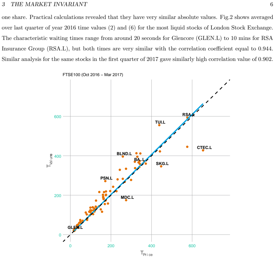
The load-bearing assertion is Eq. (8): gamma = sigma(Delta T)/<spread> * sqrt((<V_BID>+<V_ASK>)/V_Traded) * sqrt(2/(1+exp(-(<spread>/TS - 1)/sqrt(<spread>/TS)))) = 1, with the conclusion in Section 3: "Overall we could state that the market invariant (8) holds for statistical averages in a wide range of markets." If correct, volatility on a short timescale can be computed from spread, traded volume, and order book depth.

Load-bearing premise

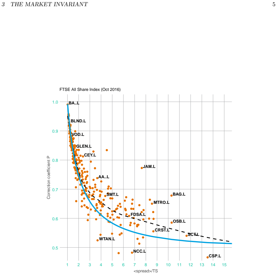
The correction coefficient P(n) in Eq. (5), whose exponential form and decay exponent -0.5 are fitted to LSE limit-order simulations (Fig. 1), is assumed to hold across venues, asset classes, and time periods. If P(n) is miscalibrated, the T_Volume estimate, the invariant, and every volatility estimate built on it are wrong. Location: Section 2.2, Eq. (5) and Fig. 1.

Share X Bluesky LinkedIn Reddit HN

Signed reviews

No signed human review yet.

Editorial analysis

A structured set of objections, weighed in public.

Desk editor's note, referee report, and a circularity audit.

Desk Editor's Note

read the letter

Colleague,

I read the Danyliv-Bland paper with interest. The headline finding—a dimensionless invariant linking volatility, spread, traded volume, and book depth—is genuinely new and has a practical feel. Equation (8) is not something I have seen in the cited literature, and the authors test it across several venues and asset classes, which is more than most microstructure papers do. The cross-exchange comparison for Barclays (Figure 3) is a nice natural experiment: the same stock on fungible venues with very different volumes gives similar instantaneous volatility estimates. That part of the paper is worth taking seriously.

The problem is the core claim. In Section 3 the authors outright reject the strong null that <γ>=1; they report no test statistic, but the rejection is unambiguous. Then they switch to a normality test, which is beside the point. A Gaussian centered at 0.85 or 1.26 can pass Shapiro-Wilk or Kolmogorov-Smirnov without supporting γ=1. And the numbers themselves tell the story: eight of nine derivative means sit below unity, and exchange averages run from 0.938 (FTSE All Share) to 1.264 (S&P/TSX). The abstract's assertion that the invariant shows no significant violation is contradicted by the paper's own significance test.

Secondary issues compound this. The correction coefficient P(n) in Eq. (5) is fitted to LSE order-flow simulations and then used to test the invariant on LSE stocks—part of the fit is self-referential. The GARCH comparison in Section 5 is not a fair one: same-day instantaneous volatility is being compared with a one-day-ahead forecast, and the one-step-ahead test in Figure 5 shows a 45% underprediction (σξ=1.454). That is a big miss for a forecasting claim.

I want to be fair: the paper is transparent about the rejection and the underprediction. It reads like an honest empirical study, not a fabrication. The underlying relation may hold approximately, and with a fitted constant it could be a useful intraday volatility proxy for execution algorithms. But the invariant claim, as stated, is not supported by the evidence.

Who should read this? Practitioners and researchers interested in microstructure-based volatility estimation will want to know the idea, even if the strict invariance fails. It deserves a serious referee because the new ratio and the cross-exchange validation are testable and worth replicating. I would send it to review, but expect the authors to either soften the claim or produce a properly calibrated version with out-of-sample tests.

My take: do not cite it as evidence for the invariant, but do look at the estimator idea.

Referee Report

4 major / 6 minor

Summary. The paper proposes a new market invariant, Eq. (8), asserting that gamma, a dimensionless combination of price volatility, spread, traded volume, and order-book depth, equals one. It then derives from this invariant an 'instantaneous volatility' estimator, Eq. (12), and compares this estimator with realised volatility and a one-day-ahead GARCH(1,1) forecast. The empirical tests cover derivatives (E-mini, crude oil, Treasury and German bond contracts) and equities from several European, Japanese, and Canadian exchanges in 2016 and early 2017. The manuscript reports that the strong null hypothesis gamma = 1 is rejected by its own significance test, and instead appeals to normality tests and to closeness of means to one. The paper concludes that the invariant holds for liquid markets and that the resulting volatility estimator is practically useful.

Significance. If the invariant were established, the paper would offer a practically valuable, microstructure-based volatility estimator requiring only short-window spreads, volumes, and order-book depth, and the cross-exchange and cross-asset empirical scope would be a useful contribution. The paper also has strengths: it directly formulates a falsifiable null hypothesis, uses high-frequency data from multiple venues, and includes a fungible-instrument check across trading venues. However, the central claim is not supported by the evidence actually presented. The paper's own statistical test rejects gamma = 1, and the fallback normality tests do not test equality to one; the correction coefficient P(n) is fitted in-sample to LSE simulations and then used for LSE stocks; the equity test uses only one quarter of data and a liquidity filter; and the GARCH comparison is not a same-horizon forecast comparison. Because Eq. (12) is derived from the rejected equality, the paper's main practical contribution inherits the unsupported claim.

major comments (4)

[Section 3, Eq. (8) and Table 1] The paper's own significance test rejects the central hypothesis. The text states that the strong null hypothesis 'gamma = 1' does not pass the statistical significance test and should be rejected, but then substitutes a weaker null hypothesis that the daily gamma values are normally distributed. Normality is irrelevant to Eq. (8): a Gaussian centred at 0.832 or 1.125 can pass the Shapiro-Wilk and Kolmogorov-Smirnov tests without supporting equality to one. Table 1 shows eight of nine derivative means below unity, with only Buxl above unity (1.125), so the abstract's claim that no significant violation of the invariant was found is contradicted by the manuscript's own test. Since Eq. (12) is obtained by setting the left side of Eq. (8) to one, the volatility estimator inherits this unsupported equality.
[Section 2.2, Eq. (5) and Fig. 1] The correction coefficient P(n) is fitted to LSE limit-order simulations and then used when testing the invariant on LSE stocks, making part of the apparent fit self-referential. The exponential form and the decay exponent -0.5 are empirical, with boundary conditions P(1)=1 and P(infinity)=1/2, but no out-of-sample validation is provided for other venues or asset classes. Because P(n) enters Eq. (6), and hence T_Volume, Eq. (8), and Eq. (12), a miscalibrated P(n) would invalidate the invariant and every volatility estimate built on it.
[Section 3, Table 2] The equity test is based on one quarter of 2016 and on a liquidity filter T_Price < 15 min, and the exchange-level averages conceal instrument-level deviations such as OMX 30 at 1.169 and S&P/TSX 60 at 1.264. Averaging over exchanges is not a joint test of gamma = 1; no test statistic for equality is reported. The statement that the invariant holds 'for statistical averages in a wide range of markets' is therefore not supported by the reported evidence.
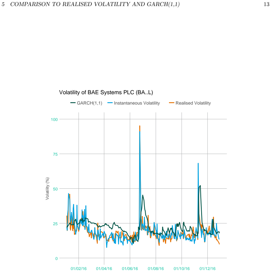
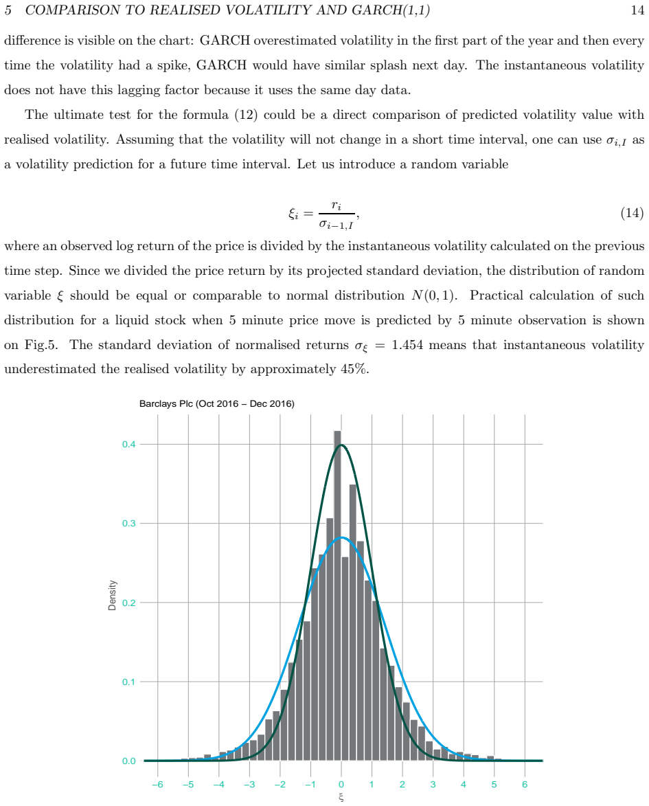
[Section 5, Eq. (13), Figs. 4 and 5] The GARCH comparison is not a same-horizon benchmark: the instantaneous volatility is computed from same-day data, whereas the one-day-ahead GARCH(1,1) forecast is made before the day begins, and the Brexit outlier is removed before computing the MSE. The reported MSE ratio is therefore not a meaningful comparison of forecasting accuracy. In addition, Fig. 5 reports sigma_xi = 1.454 for 5-minute predictions, implying an average 45% underestimation of realised volatility, which is difficult to reconcile with the claim that Eq. (8) holds with gamma = 1.

minor comments (6)

[Throughout] There are several typos and typesetting errors: 'Ki ngdom' in the author affiliation, 'T V olumre' in the Table 1 and Table 2 headers, 'Instrumens' in Table 2, and 'Andrsen' in the references.
[Eqs. (5), (8), and surrounding text] The radical notation in Eqs. (5) and (8) is garbled, with literal 'radicaltp' and 'radicalvertex' tokens that need proper mathematical typesetting.
[Section 2.2] The text states P is proportional to exp(-sqrt(n)) and then writes P(n) = 0.5(1 + exp(-(n-1)/sqrt(n))); the relationship between the proportional form and the final normalised form should be made explicit.
[Section 1] The phrase 'one tick quote and trade data' is ambiguous; the paper should clarify whether the data are top-of-book or include multiple depth levels.
[Table 3] Table 3 is based on a single stock (Barclays) and one month of observations; the claim that 5-10 minutes of history is sufficient should be caveated as a single-instrument result.
[Section 3] The 'weaker null hypothesis' is misnamed: the Shapiro-Wilk and Kolmogorov-Smirnov tests check distribution shape, not whether the mean equals one. The paper should either test mean equality directly or rename the hypothesis.

Circularity Check

0 steps flagged · score 0.0 of 10

No significant circularity; the invariant and volatility estimator are empirical, not forced by construction.

full rationale

The derivation chain is not circular in the load-bearing sense. T_Price (Eq. 2) is a random-walk characteristic time, and T_Volume (Eqs. 4-6) is a queue-depletion time with the correction coefficient P(n) calibrated to independent LSE limit-order simulations (Eq. 5, Fig. 1). The invariant gamma = 1 (Eqs. 7-8) is an empirical hypothesis, not an identity: P(n) is not chosen to make the two times equal, and the equality is tested on derivatives and multiple venues. The instantaneous volatility estimator (Eq. 12) is an algebraic rearrangement of the invariant; using an assumed invariant to derive an estimator is a legitimate application, not a tautology, and the estimator was compared with realized volatility and GARCH on data not used to fit P(n). The paper's own admission that the strong null '<gamma> = 1' fails (Section 3) is a serious internal-evidence and statistical issue, but it is not a definitional reduction or a self-referential fit. The only self-citation (Danyliv, Bland and Argenson, 2015) supports an interpretive 32% probability for T_Price and is not load-bearing. The reuse of the LSE-calibrated P(n) in the LSE portion of the invariant test is an in-sample overfitting concern, but it does not force gamma = 1 by construction, so it does not amount to circularity.

Assumptions & free parameters 3 free parameters · 5 assumptions · 0 invented entities

The central claim rests on two heuristic characteristic times, a fitted correction coefficient, and several equilibrium/random-walk approximations. No genuinely new physical or economic entity is introduced; the 'invariant' is a relation among existing observables. The main uncharged inputs are the functional form of P(n) and the three data-selection thresholds.

free parameters (3)

Decay exponent in correction coefficient P(n) = -0.5 (exponent applied to sqrt(n) in Eq. (5))
The exponential decay form and the -0.5 power are fitted to LSE limit-order simulation data in Section 2.2; this is a hand/fitted constant used in T_Volume and hence in the invariant.
Equity liquidity filter threshold = 15 min T_Price
Section 3 selects only stocks with characteristic time T_Price < 15 min; this choice affects which instruments are included in the invariant tests and the measured averages.
Derivative day volume filter = 20% of maximum observed volume
Section 3 keeps only days with trading volume higher than 20% of the max for each futures contract, which determines the construction of the derivatives data sets.

assumptions (5)

domain assumption Price follows a random walk with square-root time scaling for volatility.
Section 2.1, Eq. (1) uses this to derive T_Price; if the price process has memory or jumps, T_Price is not the characteristic time.
domain assumption In equilibrium, half of traded volume occurs on the bid side and half on the ask side.
Section 2.2, Eq. (3) uses this to split V_Traded into one side; order flow imbalance can violate it.
ad hoc to paper The probability of a trade participating in queue depletion decays exponentially with distance from the touch, with boundary values P(1)=1 and P(infinity)=1/2.
Section 2.2, Eq. (5); the functional form is fitted to simulations, not derived.
domain assumption Realised volatility can be approximated by the standard deviation of price divided by average price, with overnight returns omitted.
Section 3, Eqs. (9)-(10) use this approximation; opening gaps and price jumps can bias realized volatility.
domain assumption Volatility is locally persistent, so the previous interval's estimate forecasts the next interval.
Section 5, Eq. (14) uses the previous 5-minute estimate to standardize the next return; this persistence is the null assumption of the forecast test, and the realized sigma_xi=1.454 shows it is only approximate.

how reviews work

0 comments

Cite this review

Pith. "Pith review of An instantaneous market volatility estimation." pith.science (2026). https://pith.science/paper/Q6YWLIOU

@misc{pith2026190802847,
  author       = {Pith},
  title        = {Pith review of: An instantaneous market volatility estimation},
  year         = {2026},
  howpublished = {\url{https://pith.science/paper/Q6YWLIOU}},
  note         = {Machine review of arXiv:1908.02847}
}

read the original abstract

Working on different aspects of algorithmic trading we empirically discovered a new market invariant. It links together the volatility of the instrument with its traded volume, the average spread and the volume in the order book. The invariant has been tested on different markets and different asset classes. In all cases we did not find significant violation of the invariant. The formula for the invariant was used for the volatility estimation, which we called the instantaneous volatility. Quantitative comparison showed that it reproduces realised volatility better than one-day-ahead GARCH(1,1) prediction. Because of the short-term prediction nature, the instantaneous volatility could be used by algo developers, volatility traders and other market professionals.

Figures

Figures reproduced from arXiv: 1908.02847 by the authors.

**Figure 2.** Times TV olume and TP rice in seconds for stocks of FTSE100. Each orange dot corresponds to the individual instrument. Dashed line is a diagonal line, solid blue line corresponds to the regression line from forced to cross (0,0) point. Using these observations, one can assume that the following invariant is present on the market γ 2 ≡ TV olume TP rice = 1. (7) The square root of this ratio will depend linearly from … view at source ↗

**Figure 3.** The instantaneous volatility for Barclays PLC, ca [PITH_FULL_IMAGE:figures/full_fig_p011_3.png] view at source ↗

Figures from the paper (2 more)

**Figure 4.** Figure 4: BA..L realised volatility (orange line) compared [PITH_FULL_IMAGE:figures/full_fig_p013_4.png]

**Figure 5.** Figure 5: The distribution of random variable ξi when historical 5 min data was used to predict standard deviation of next 5 min price return. Blue line represents the fitted normal distribution with σ(ξ) = 1.454, green line is N(0, 1) distribution [PITH_FULL_IMAGE:figures/full…

Discussion (0). Continue with ORCID to comment.

Reference graph

Works this paper leans on

8 extracted references · 8 canonical work pages

[1]

author S. Figlewski , title Forecasting Volatility Using Historical Data , title Finance Department, Working Paper Series , publisher New York University, Stern School of Business , address New York, NY , ( year 1994 )

work page 1994
[2]

Andrsen , author T

author T.G. Andrsen , author T. Bollerslev , author F.X. Diebold , author H. Ebens , title The distribution of relized stock return volatility , journal Journal of Financial Economics volume 61 ( year 2001 ), pages 43--76

work page 2001
[3]

Danyliv , author B

author O. Danyliv , author B. Bland , author A. Argenson , title Random walk model from the point of view of algorithmic trading , journal SSRN, https://ssrn.com/abstract=3436367

work page
[4]

Brownlees , author R

author C. Brownlees , author R. Engle , author B. Kelly , title A practical guide to volatility forecasting through calm and storm , journal The Journal of Risk volume 14 number 2 ( year 2011 ), pages 3--22

work page 2011
[5]

Wuertz , title R Package 'fGarch' , version ver 3010.82.1 ( year 2013 ), link https://cran.r-project.org/web/packages/fGarch/fGarch.pdf

author D. Wuertz , title R Package 'fGarch' , version ver 3010.82.1 ( year 2013 ), link https://cran.r-project.org/web/packages/fGarch/fGarch.pdf

work page 2013
[6]

Bogousslavsky , author P

author V. Bogousslavsky , author P. Collin-Dufresne , title Liquidity, Volume and Volatility , journal SSRN, https://ssrn.com/abstract=3336171 ( year 2019 )

work page 2019
[7]

Andersen , author T

author T.G. Andersen , author T. Bollerslev , author F.X. Diebold , author P. Labys , title Exchange Rate Returns Standardized by Realized Volatility are (Nearly) Gaussian , journal Multinational Finance Journal volume 4 , number no. 3&4 ( year 2000 ), pages 159--179

work page 2000
[8]

Koopman , author B

author S.J. Koopman , author B. Jungbacker , author E. Hol , title Forecasting Daily Variability of the S&P 100 Stock Index Using Historical, Realised and Implied Volatility Measurements , journal Tinbergen Institute Working Paper , volume 016 , number 4 ( year 2004 ), link SSRN, https://papers.ssrn.com/sol3/papers.cfm/abstract=499744

work page 2004

Pith tools

Reviewed August 14, 2026 · model on record in the stance chip above.

[1] [1]

author S. Figlewski , title Forecasting Volatility Using Historical Data , title Finance Department, Working Paper Series , publisher New York University, Stern School of Business , address New York, NY , ( year 1994 )

work page 1994

[2] [2]

Andrsen , author T

author T.G. Andrsen , author T. Bollerslev , author F.X. Diebold , author H. Ebens , title The distribution of relized stock return volatility , journal Journal of Financial Economics volume 61 ( year 2001 ), pages 43--76

work page 2001

[3] [3]

Danyliv , author B

author O. Danyliv , author B. Bland , author A. Argenson , title Random walk model from the point of view of algorithmic trading , journal SSRN, https://ssrn.com/abstract=3436367

work page

[4] [4]

Brownlees , author R

author C. Brownlees , author R. Engle , author B. Kelly , title A practical guide to volatility forecasting through calm and storm , journal The Journal of Risk volume 14 number 2 ( year 2011 ), pages 3--22

work page 2011

[5] [5]

Wuertz , title R Package 'fGarch' , version ver 3010.82.1 ( year 2013 ), link https://cran.r-project.org/web/packages/fGarch/fGarch.pdf

author D. Wuertz , title R Package 'fGarch' , version ver 3010.82.1 ( year 2013 ), link https://cran.r-project.org/web/packages/fGarch/fGarch.pdf

work page 2013

[6] [6]

Bogousslavsky , author P

author V. Bogousslavsky , author P. Collin-Dufresne , title Liquidity, Volume and Volatility , journal SSRN, https://ssrn.com/abstract=3336171 ( year 2019 )

work page 2019

[7] [7]

Andersen , author T

author T.G. Andersen , author T. Bollerslev , author F.X. Diebold , author P. Labys , title Exchange Rate Returns Standardized by Realized Volatility are (Nearly) Gaussian , journal Multinational Finance Journal volume 4 , number no. 3&4 ( year 2000 ), pages 159--179

work page 2000

[8] [8]

Koopman , author B

author S.J. Koopman , author B. Jungbacker , author E. Hol , title Forecasting Daily Variability of the S&P 100 Stock Index Using Historical, Realised and Implied Volatility Measurements , journal Tinbergen Institute Working Paper , volume 016 , number 4 ( year 2004 ), link SSRN, https://papers.ssrn.com/sol3/papers.cfm/abstract=499744

work page 2004