REVIEW 1 major objections 6 minor 42 references
3D Compton scattering imaging: study of the spectrum and contour reconstruction
T0 review · 1 major / 6 minor · reviewed 2026-08-14 · deepseek-v4-flash
Pith's one-line read 3D Compton scattering imaging can recover electron-density contours from a mixed first- and second-order spectrum, because linearized second-order scattering is a smoother Fourier integral operator ($-7/4$ vs $-1$).
desk verdict Real new math for second-order Compton scattering (g2 integral representation and the -7/4 vs -1 FIO order gap), with an honest but real gap between the linearized smoothness theorem and the contour-reconstruction claim; worth refereeing, not desk-rejecting. read the letter →
The pith
A machine-rendered reading of the paper's core claim, the machinery that carries it, and where it could break.
The reading
What carries the argument
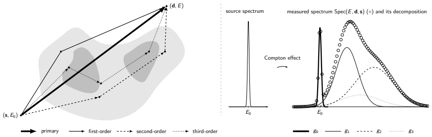
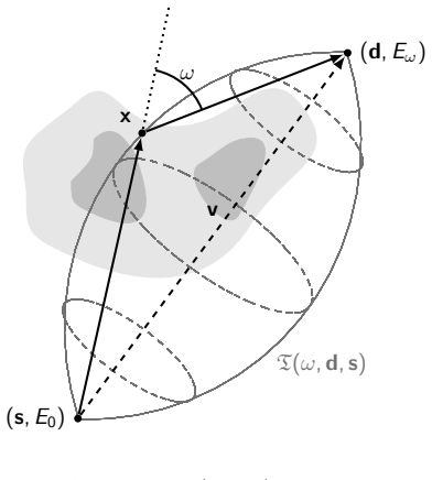
The load-bearing machinery is a pair of linearized Fourier integral operators. $L_1$ is the weighted toric Radon transform of the first-order model, with phase $\varphi(x,d,s)$ selecting spindle tori, the surfaces of points from which a photon can reach the detector after one scattering. $L_2$ is built from the intersection of a cone and a spindle torus, with phase $\Psi(y,x,d,s)$ coming from the two-angle Compton relation; its integration runs over the six-dimensional pair $(x,y)$ of first and second scattering points. The FIO order is computed from the phase dimensions, $m=\frac{1}{2}-\frac{3+3}{4}=-1$ for $L_1$ and $m=\frac{1}{2}-\frac{6+3}{4}=-\frac{7}{4}$ for $L_2$, and the Sobolev smoothing statements follow from standard microlocal immersion conditions on the detector manifold. The nondegeneracy proof for the $L_2$ phase uses the fact that $\nabla_y\Psi\cdot(y-x)\neq 0$ when the two scattering points are distinct.
What would settle it
Compute $g_1$ and $g_2$ from a phantom with a sharp edge, using either the paper's analytic models or Monte-Carlo simulation, and apply formula (27) to $g_1$ alone and to $g_1+g_2$. If the gradients from the combined data show edge-like features with amplitude comparable to the true contours, or if the Fourier power spectrum of $g_2$ does not decay faster than that of $g_1$ by the predicted $3/4$ Sobolev order, the central claim is false.
Extended reading notes
Core claim
The central claim is Theorem 3.6: the linearized second-order scattering operator $L_2$ lies in $I^{-7/4}(\mathbb{R}\times D,\Omega_2)$, while the linearized first-order operator $L_1$ lies in $I^{-1}(\mathbb{R}\times D,\Omega)$ (Theorem 3.5). Under the immersion conditions of Lemma 3.7 and Corollary 3.9 this translates into Sobolev continuity with one full derivative of smoothing for $L_1$ and $7/4$ (at least $5/4$) for $L_2$. Hence the singular part of the spectrum, the contours of the electron density, is carried essentially by the first-order radiation, and the reconstruction formula $\tilde{f}=B\partial_p^2(g_1+g_2+\eta)$, with $B$ the weighted dual operator, recovers contours without an explicit model for $g_2$. The paper presents this as the reason contour-based imaging can use multiple-scattered data, and validates it with synthetic and Monte-Carlo simulations.
Load-bearing premise
The argument assumes the true electron density background is infinitely smooth and replaces the real nonlinear measurement by a linearized operator; if the background is only piecewise smooth, or if the neglected weight singularities are not subordinate, the second-order term could hide contours at the same strength as the signal.
Editorial extensions
If this is right
- Contour reconstructions can be computed from the raw spectrum $g_1+g_2+\eta$ using only the first-order filtered backprojection (26)-(27); no model or estimate of $g_2$ is needed in the algorithm.
- Scanner geometry must satisfy condition (23) and the non-vanishing determinant of Lemma 3.7; otherwise the backprojection weight $h(x,d)$ degenerates and the immersion property fails.
- The order gap quantifies why a second derivative in the spectral variable works: it amplifies the order $-1$ part while the order $-7/4$ part remains comparatively smooth.
- Conjecture 3.10 predicts that each additional scattering order lowers the FIO order by another $3/4$, so the same contour extraction should tolerate higher-order scattering as smooth background.
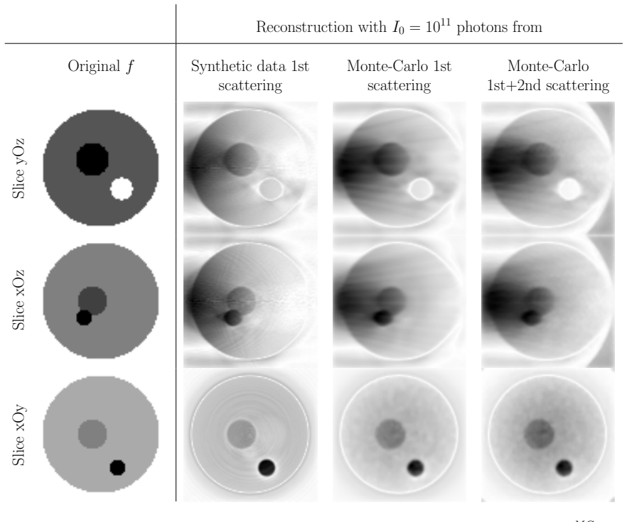
- Synthetic and Monte-Carlo tests with 0.5% Poisson noise show that the gradient of the reconstruction from $g_1+g_2$ keeps the edges visible, not just the gradient from $g_1$ alone.
Reading between the lines
- Editorial inference: a direct spectral test is available—if the Fourier/wavelet coefficients of $g_2$ do not decay faster than those of $g_1$, the predicted $3/4$ Sobolev gap is absent and the contour argument would need revision.
- Editorial inference: because the proof linearizes around a smooth background, a piecewise-constant phantom is the natural stress test; robustness of formula (27) at a sharp interface is not covered by the proof and would determine practical applicability.
- Editorial inference: the same order-gap reasoning suggests that finite energy resolution in real detectors acts as an additional smoothing comparable to $g_2$, so contour extraction should tolerate coarse energy bins as long as the bin width does not smooth $g_1$ down to the $g_2$ level.
Signed reviews
Editorial analysis
A structured set of objections, weighed in public.
Referee Report
Summary. The paper studies 3D Compton scattering imaging with a monochromatic external source and energy-resolving detectors. Section 2 gives integral representations for the measured spectrum: first-order scattering g1 is modeled as a weighted toric Radon transform T(ne) (Eq. (7)), and second-order scattering g2 is modeled as the double-scattering operator S(ne) (Theorem 2.1, Eqs. (15) and (17)), with qualitative validation against Monte-Carlo data (Section 2.3). Section 3 replaces T and S by linearized operators L1 and L2 (Eqs. (18) and (19)) and proves, under the hypothesis ne in C^infty(Omega), that L1 is a Fourier integral operator of order -1 (Theorem 3.5) and that L2 is a Fourier integral operator of order -7/4 (Theorem 3.6); Sobolev continuity under detector conditions follows in Corollaries 3.8 and 3.9. Section 4 applies the first-order filtered-backprojection-type reconstruction B d_p^2 to the mixed spectrum g1+g2+eta (Eqs. (26) and (27)) and presents contour reconstructions from synthetic and Monte-Carlo data. The central claim is that second-order scattered radiation is structurally smoother than first-order radiation, so that the contours of the electron density are encoded in the first-order part and can be recovered from g1+g2 without explicitly modeling g2.
Significance. The paper contains a useful, largely self-contained derivation of the second-order forward model and a plausible FIO-order computation for the linearized operators L1 and L2. If the smoothness comparison could be rigorously transferred from the linearized operators to the actual nonlinear measurement operators T(ne) and S(ne), the conclusion would be practically significant, because it would justify contour imaging from raw multi-scatter spectra without modeling g2. The manuscript is honest about several deferred points, but those deferrals concern exactly the load-bearing step that connects Theorem 3.6 to the reconstruction claims. The numerical results are qualitative and rely on a smooth prior density in the reconstruction kernel, so they are suggestive rather than conclusive. The paper also gives a concrete detector condition (Lemma 3.7) and validates the forward models, which are positive elements of the contribution.
major comments (1)
- [Section 3.2, Theorem 3.6, and Section 4] The paper asserts that the reconstruction operator in Eq. (26) acts as an FIO of order 1 and concludes from this that the second derivative d_p^2 highlights g1 over g2, but no microlocal estimate is given for the composition B d_p^2 L2 or for the action of this composition on the residual R. A Sobolev gain of 7/4 for L2 (or 5/4 in the degenerate case of Corollary 3.9) does not by itself determine whether the contour information from g1 dominates after the order-2 differentiation and the order-1 backprojection; a quantitative statement, such as the FIO order of B d_p^2 L2 relative to B d_p^2 L1, is needed to support the reconstruction claim. The heuristic statement in Section 4 that d_p^2 'highlights the variations of g1 over g2' should be replaced or supplemented by such an estimate.
minor comments (6)
- [Section 2.1, Eq. (1)] The line beginning with the logarithm of the intensity ratio is typeset in a confusing way; the displayed formula should be cleaned up so that the definition g(s,theta)=R mu_E(s,theta) appears without the misplaced equality and parentheses.
- [Abstract] The phrase 'to argument why and how' should read 'to argue why and how'.
- [Section 3.1, proof of Theorem 3.6] In the nondegeneracy argument, the symbol Phi is used where Upsilon is meant; the displayed expression for the derivative of d_sigma Upsilon should depend on Psi, and the notation should be corrected.
- [Section 2.3] The text refers to 'the intersection between torus and cylinder' for the second-order scattering, but the intersection is between the cone C(omega1,x,s) and the spindle torus T(omega2,d,x); this should be corrected.
- [Definition 1.1] The formula for the order of a Fourier integral operator is typeset ambiguously as 's - n + m - 2 / 4'; it should be written as s - (n+m-2)/4 to match the computations in Theorems 3.5 and 3.6.
- [Conjecture 3.10 and Conclusion] The abstract and conclusion present the second-order smoothness and the contour-reconstruction claim as established facts, while the body states that several parts of the microlocal analysis are deferred to future research; adding a caveat in the abstract or conclusion would make the paper more accurate about the status of the claims.
Circularity Check
The derivation is essentially self-contained; the smoothness comparison is a genuine FIO computation, not a renamed input.
full rationale
The paper's central claim is that the second-order scattered radiation is structurally smoother than the first-order part, quantified by FIO orders -7/4 versus -1 (Theorems 3.5 and 3.6). The chain leading to this claim is not circular: the integral representation of g2 is derived from the Compton formula, Klein-Nishina scattering, Beer-Lambert attenuation, and an explicit geometric intersection of a cone and spindle torus (Theorem 2.1); the linearized operators L1 and L2 are then analyzed with standard microlocal tools. The order difference is a computed consequence of the phase dimension (6-dimensional fiber for L2 versus 3-dimensional for L1), not an assumption equivalent to the conclusion. The paper relies on the author's prior toric Radon transform model and inversion formula [35], but that is published prior work used as a starting point, and the new smoothness comparison does not reduce to it. No fitted parameter is renamed as a prediction, and no target quantity is defined in terms of its own outcome. The main caveat is that the contour-reconstruction claim for the actual nonlinear measurement S(ne) with discontinuous ne is explicitly deferred ('This intuition will be the core of future researches'), and the microlocal transfer from smooth linearized operators to non-smooth truth is unproven; this is a correctness/validity limitation, not circularity. Self-citations are present but are not load-bearing in a circular way, hence the low score.
Assumptions & free parameters
assumptions (5)
- standard math Standard theory of Fourier integral operators and Sobolev estimates, including Hörmander [19] and Krishnan-Quinto [22], is used as an unproved background tool.
- domain assumption The physics of Compton scattering: Compton formula (3), Klein-Nishina probability, Beer-Lambert attenuation with photoelectric term, and photometric dispersion model the measured radiation.
- domain assumption Scattering of order three and higher is neglected and treated as noise.
- domain assumption For the FIO analysis, the electron density ne is assumed C∞ and compactly supported, and the true operators T and S are replaced by linearized operators L1 and L2.
- domain assumption The detector geometry satisfies the immersion conditions of Lemma 3.7, including eq. (23) and the condition h(x,d)≠0.
Cite this review
Pith. "Pith review of 3D Compton scattering imaging: study of the spectrum and contour reconstruction." pith.science (2026). https://pith.science/paper/3CZMVWE4
@misc{pith2026190803066,
  author       = {Pith},
  title        = {Pith review of: 3D Compton scattering imaging: study of the spectrum and contour reconstruction},
  year         = {2026},
  howpublished = {\url{https://pith.science/paper/3CZMVWE4}},
  note         = {Machine review of arXiv:1908.03066}
}
read the original abstract
3D Compton scattering imaging is an upcoming concept exploiting the scattering of photons induced by the electronic structure of the object under study. The so-called Compton scattering rules the collision of particles with electrons and describes their energy loss after scattering. Although physically relevant, multiple-order scattering was so far not considered and therefore, only first-order scattering is generally assumed in the literature. The purpose of this work is to argument why and how a contour reconstruction of the electron density map from scattered measurement composed of first- and second-order scattering is possible (scattering of higher orders is here neglected). After the development of integral representations for the first- and second-order scattering, this is achieved by the study of the smoothness properties of associated Fourier integral operators (FIO). The second-order scattered radiation reveals itself to be structurally smoother than the radiation of first-order indicating that the contours of the electron density are essentially encoded within the first-order part. This opens the way to contour-based reconstruction techniques when using multiple scattered data. Our main results, modeling and reconstruction scheme, are successfully implemented on synthetic and Monte-Carlo data.
Figures

Figures from the paper (8 more)




Reference graph
Works this paper leans on
-
[1]
O. O. Adejumo, F. A. Balogun, and G. G. O. Egbedokun , Developing a compton scattering tomography system for soil studies: Theory, Journal of Sustainable Development and Environmen- tal Protection, 1 (2011), pp. 73–81
work page 2011
-
[2]
R. Al v arez and A. Macovski, Energy-selective reconstructions in x-ray computerized tomog- raphy, Phys Med Biol., 21 (1976), pp. pp. 733–744
work page 1976
-
[3]
S. Anghaie, L. L. Humphries, and N. J. Diaz , Material characterization and flaw detection, sizing, and location by the differential gamma scattering spectroscopy technique. Part1: Develop- ment of theoretical basis, Nuclear Technology, 91 (1990), pp. 361–375
work page 1990
-
[4]
N. V. Arendtsz and E. M. A. Hussein , Energy-spectral Compton scatter Imaging - Part 1: theory and mathematics, IEEE Transactions on Nuclear Sciences, 42 (1995), pp. 2155–2165
work page 1995
-
[5]
F. A. Balogun and P. E. Cruvinel , Compton scattering tomography in soil compaction study, Nuclear Instruments and Methods in Physics Research A, 505 (2003), pp. 502–507
work page 2003
-
[6]
A. Brunetti, R. Cesareo, B. Golosio, P. Luciano, and A. Ruggero , Cork quality esti- mation by using Compton tomography, Nuclear instruments and methods in Physics research B, 196 (2002), pp. 161–168
work page 2002
-
[7]
R. Cesareo, C. C. Borlino, A. Brunetti, B. Golosio, and A. Castellano , A simple scanner for Compton tomography, Nuclear Instruments and Methods in Physics Research A, 487 (2002), pp. 188–192
work page 2002
-
[8]
R. L. Clarke and G. V. Dyk , A new method for measurement of bone mineral content using both transmitted and scattered beams of gamma-rays, Phys. Med. Biol., 18 (1973), pp. 532–539
work page 1973
Show all 42 references
-
[9]
A. H. Compton , A quantum theory of the scattering of x-rays by light elements, Phys. Rev., 21 (1923), pp. 483–502
1923
-
[10]
Driol , Imagerie par rayonnement gamma diffusé à haute sensibilité, PhD thesis, Univ
C. Driol , Imagerie par rayonnement gamma diffusé à haute sensibilité, PhD thesis, Univ. of Cergy-Pontoise, 2008. 26
2008
-
[11]
Shefer et al, State of the Art of CT Detectors and Sources: A Literature Review, Current Radiology Reports, 1 (2013), pp
E. Shefer et al, State of the Art of CT Detectors and Sources: A Literature Review, Current Radiology Reports, 1 (2013), pp. pp. 76–91
2013
-
[12]
B. L. Ev ans, J. B. Martin, L. W. Burggraf, and M. C. Roggemann , Nondestructive inspection using Compton scatter tomography, IEEE Transactions on Nuclear Science, 45 (1998), pp. 950–956
1998
-
[13]
F. T. F armer and M. P. Collins , A new approach to the determination of anatomical cross- sections of the body by Compton scattering of gamma-rays, Phys. Med. Biol., 16 (1971), pp. 577– 586
1971
-
[14]
Fredenberg, Spectral and dual-energy X-ray imaging for medical applications
E. Fredenberg, Spectral and dual-energy X-ray imaging for medical applications. Nuclear In- struments and Methods in Physics Research Section A: Accelerators, Spectrometers, Detectors and Associated Equipment, 878 (2018), pp. pp 74–87
2018
-
[15]
Goo and J
H. Goo and J. Goo , Dual-Energy CT: New Horizon in Medical Imaging, Korean J Radiol., 18 (2017), pp. pp. 555–569
2017
-
[16]
V. A. Gorshkov, M. Kroening, Y. V. Anosov, and O. Dorjgochoo , X-Ray scattering tomography, Nondestructive Testing and Evaluation, 20 (2005), pp. 147–157
2005
-
[17]
Guzzardi and G
R. Guzzardi and G. Licitra , A critical review of Compton imaging, CRC Critical Reviews in Biomedical Imaging, 15 (1988), pp. 237–268
1988
-
[18]
Harding and E
G. Harding and E. Harding , Compton scatter imaging: a tool for historical exploitation, Appl Radiat Isot., 68 (2010), pp. 993–1005
2010
-
[19]
Hörmander, Fourier Integral Operators, I, vol
L. Hörmander, Fourier Integral Operators, I, vol. 127, Acta Math., 1971
1971
-
[20]
Hounsfield, Computerized transverse axial scanning (tomography)
G. Hounsfield, Computerized transverse axial scanning (tomography). i. description of system, Br J Radiol., 46 (1973), pp. pp. 1016–1022
1973
-
[21]
Klein and Y
O. Klein and Y. Nishina , Über die Streuung von Strahlung durch freie Elektronen nach der neuen relativistischen Quantendynamik von Dirac, Z. Phys., 52 (1929), pp. 853–869
1929
-
[22]
Krishnan and E
V. Krishnan and E. T. Quinto , Microlocal Analysis in Tomography, Handbook of Mathemat- ical Methods in Imaging, Book editor: Otmar Scherzer, 2015
2015
-
[23]
Kuchment, K
P. Kuchment, K. Lancaster, and L. Mogilevskaya ,On local tomography, InverseProblems, 11 (1995), p. 571
1995
-
[24]
P. G. Lale , The Examination of Internal Tissues, using Gamma-ray Scatter with a Possible Extension to Megavoltage Radiography, Physics in Medicine and Biology, 4 (1959), pp. 159–167
1959
-
[25]
A. K. Louis , Approximate inverse for linear and some nonlinear problems, Inverse Problems, 12 (1996), pp. 175–190
1996
-
[26]
McCollough, S
C. McCollough, S. Leng, Y. Lifeng, and J. Fletcher , Dual- and Multi-Energy CT: Principles, Technical Approaches, and Clinical Applications, Radiology, 276 (2015), pp. pp. 637– 653
2015
-
[27]
D. A. Meneley, E. M. A. Hussein, and S. Banerjee , On the solution of the inverse problem of radiation scattering imaging, Nuclear Science and Engineering, 92 (1986), pp. 341–349
1986
-
[28]
Natterer, The mathematics of computerized tomography, 2001
F. Natterer, The mathematics of computerized tomography, 2001
2001
-
[29]
Nguyen, T
M. Nguyen, T. Truong, M. Mor vidone, and H. Zaidi , Scattered radiation emission imaging: Principles and applications, International Journal of Biomedical Imaging (IJBI), (2011), p. 15pp. 27
2011
-
[30]
S. J. Norton , Compton scattering tomography, Jour. Appl. Phys., 76 (1994), pp. 2007–2015
1994
-
[31]
Palamodov, A uniform reconstruction formula in integral geometry, Inverse Problems, 28 (2012), p
V. Palamodov, A uniform reconstruction formula in integral geometry, Inverse Problems, 28 (2012), p. 065014
2012
-
[32]
Prado, M
P. Prado, M. Nguyen, L. Dumas, and S. Cohen , Three-dimensional imaging of flat natural and cultural heritage objects by a Compton scattering modality, Journal of Electronic Imaging, 26 (2017), p. 011026
2017
-
[33]
Primak, J
A. Primak, J. R. Giraldo, X. Liu, L. Yu, and C. McCollough , Improved dual-energy material discrimination for dual-source CT by means of additional spectral filtration, Med Phys., 36 (2009), pp. pp. 1359–1369
2009
-
[34]
Rigaud, Compton Scattering Tomography: Feature Reconstruction and Rotation-Free Modal- ity, SIAM J
G. Rigaud, Compton Scattering Tomography: Feature Reconstruction and Rotation-Free Modal- ity, SIAM J. Imaging Sci., 10 (2017), p. 2217–2249
2017
-
[35]
Rigaud and B
G. Rigaud and B. Hahn , 3D Compton scattering imaging and contour reconstruction for a class of Radon transforms, Inverse Problems, 2018 (7), p. 075004
2018
-
[36]
Rigaud and A
G. Rigaud and A. Lakhal , Approximate inverse and Sobolev estimates for the attenuated Radon transform, Inverse Problems, 31 (2015), p. 105010
2015
-
[37]
J. P. Stonestrom, R. E. Al v arez, and A. Macovski , A framework for spectral artifact corrections in x-ray CT, IEEE Trans. Biomed. Eng., 28 (1981), pp. 128–141
1981
-
[38]
Tracey and E
B. Tracey and E. Miller , Stabilizing dual-energy X-ray computed tomography reconstructions using patch-based regularization, Inverse Problems, 31 (2015), p. 05004
2015
-
[39]
Webber and S
J. Webber and S. Holman , Microlocal analysis of a spindle transform, arXiv e-prints, (2017), arXiv:1706.03168, p. arXiv:1706.03168,https://arxiv.org/abs/1706.03168
2017 arXiv
-
[40]
Webber and W
J. Webber and W. Lionheart , Three dimensional Compton scattering tomography, arXiv e- prints, (2017), arXiv:1704.03378, p. arXiv:1704.03378,https://arxiv.org/abs/1704.03378
2017 arXiv
-
[41]
Webber and E
J. Webber and E. Quinto , Microlocal analysis of a Compton tomography problem, arXiv e- prints, (2019), arXiv:1902.09623, p. arXiv:1902.09623,https://arxiv.org/abs/1902.09623
2019 arXiv
-
[42]
Weisstein, Spindle torus, From MathWorld–A Wolfram Web Resource,http://mathworld
E. Weisstein, Spindle torus, From MathWorld–A Wolfram Web Resource,http://mathworld. wolfram.com/SpindleTorus.html. 28
Reviewed August 14, 2026 · model on record in the stance chip above.
Discussion (0). Continue with ORCID to comment.