REVIEW 2 major objections 4 minor 34 references
A second-order face-centred finite volume method for elliptic problems
T0 review · 2 major / 4 minor · reviewed 2026-08-14 · deepseek-v4-flash
Pith's one-line read The paper claims a second-order face-centred finite volume method for elliptic problems that solves a global system identical in size and sparsity to the first-order method.
desk verdict A solid, practically useful second-order extension of FCFV whose theoretical inheritance from Oikawa's reduced-stabilisation HDG is legitimate, though the paper would benefit from a sharper statement of that link and an independent baseline. read the letter →
The pith
A machine-rendered reading of the paper's core claim, the machinery that carries it, and where it could break.
The reading
What carries the argument
The key mechanism is a projection operator $P_0$ placed inside the numerical flux: on each face the flux is $n\cdot q_h + \tau_e(P_0 u_h - \hat u)$ (with Dirichlet data in place of $\hat u$ on the Dirichlet boundary). $P_0$ sends the linear in-cell solution to its constant average on the face, and it is the single ingredient that turns the first-order face-centred method into a second-order one. The paper proves in Lemma 1 that $\int_{\Gamma_{e,i}} P_0 u_h\,d\Gamma = \int_{\Gamma_{e,i}} u_h\,d\Gamma$, so the projection only changes the cell-level matrix $m_e$ and leaves the global system's size and sparsity untouched. The rest of the machinery is the standard HDG/FCFV split: a local Dirichlet problem per element eliminates the interior solution and gradient in terms of the face unknowns, and the global problem enforces flux continuity on the faces.
What would settle it
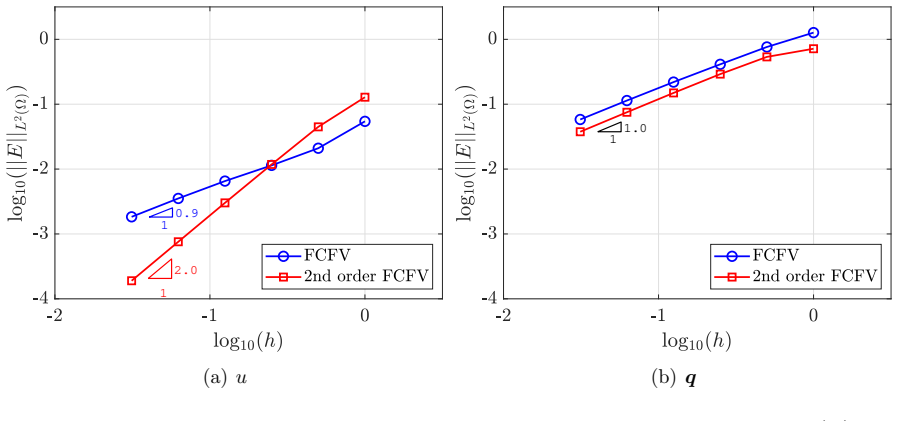
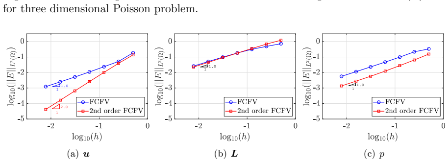
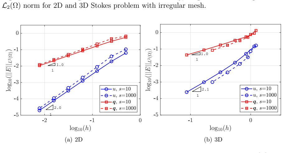
Solve the Poisson problem on a sequence of tetrahedral meshes with stretching factor 1000 as in Section 5.5, and compute the relative $L^2$ error of the solution against the exact solution. If the measured convergence order is not close to 2 (or if it degrades with mesh distortion), the paper's central claim of second-order accuracy at a first-order global cost fails; the paper's own Figures 10 and 12 are the evidence it would need to match.
Extended reading notes
Core claim
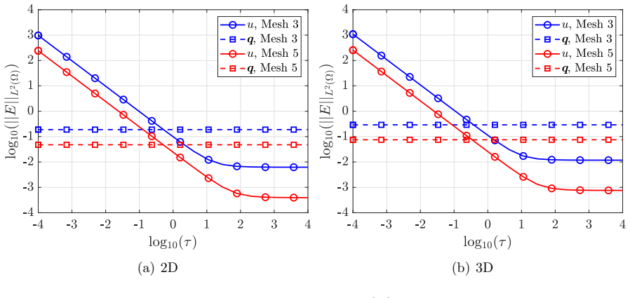
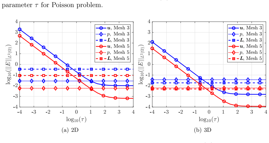
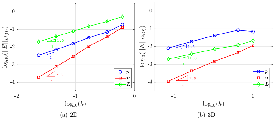
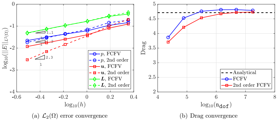
The paper claims that a face-centred finite volume method, which stores the unknown on mesh faces and treats the gradient as an independent variable, can be upgraded from first to second order convergence in the solution without enlarging the globally coupled system. The construction follows hybridised discontinuous Galerkin methods with reduced stabilisation: inside each cell the solution is approximated by a linear polynomial, while the gradient and the face unknowns are piecewise constant, and the numerical flux contains a projection of the cell solution onto constants. Removing that projection collapses the method back to first order, which is precisely why the difference between the two variants can be used as an error indicator. The global system, whose unknowns are the face values, is claimed to have the same size and the same number of non-zero entries as the first-order method because the face space is unchanged. Numerical experiments show second-order convergence for the solution, first-order convergence for the gradient, the same rates on distorted and stretched meshes, and for Stokes flow the method passes the LBB condition and delivers second-order velocity and first-order pressure convergence.
Load-bearing premise
The paper relies on the assumption that the mathematical analysis of a related, more general family of methods carries over to this particular face-centred scheme, including on highly distorted and stretched meshes; it does not prove that carry-over itself.
Editorial extensions
If this is right
- For a given mesh, the solution error drops from first to second order with no extra global unknowns, so a target accuracy is reached with far fewer degrees of freedom.
- Because the gradient is a direct unknown, no reconstruction step is needed, and the method keeps its convergence rates on strongly distorted and stretched meshes.
- The global linear system has the same size and non-zero pattern as the first-order method, so the extra accuracy is obtained at essentially the same assembly and solve cost per mesh.
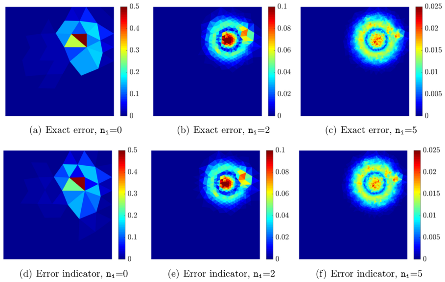
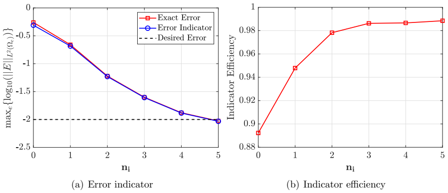
- The difference between the first- and second-order solutions gives a computable error indicator that drives h-adaptivity without solving an auxiliary problem.
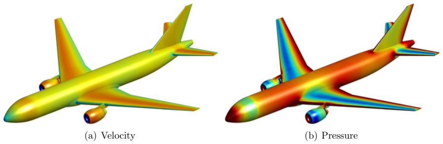
- For Stokes flows, the method preserves the LBB condition and gives second-order velocity, first-order pressure and gradient; the paper demonstrates this in problems with over 5 million tetrahedra.
Reading between the lines
- The same device should extend to higher-order face-centred methods: using degree-$k$ polynomials inside cells with a projection onto the trace space would likely reproduce the HDG convergence hierarchy while keeping the face unknowns fixed, so the global cost would remain tied to the face space rather than the interior order.
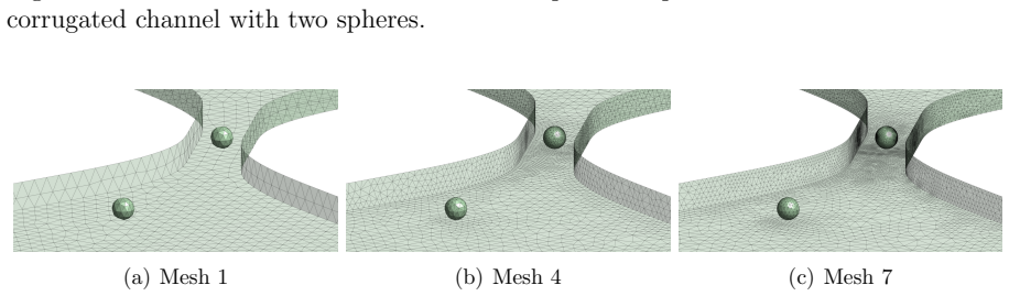
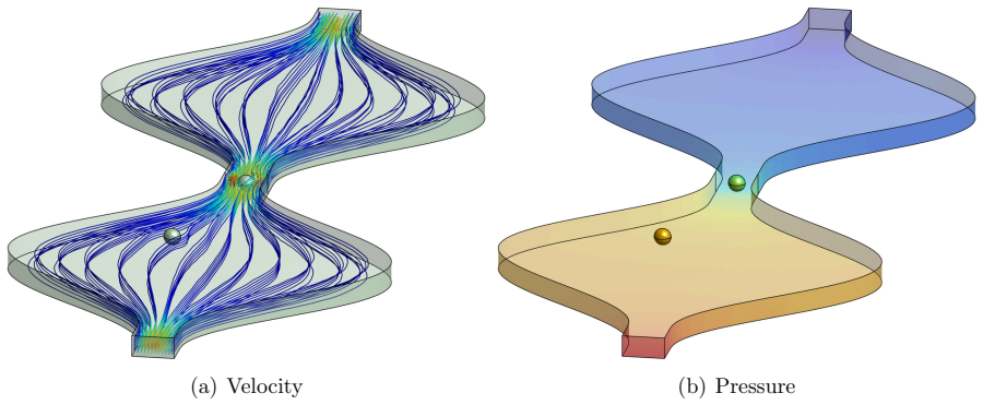
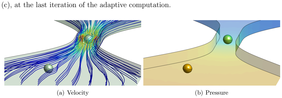
- The cheap error indicator suggests an industrial-grade adaptive strategy: run the first- and second-order variants simultaneously, use their difference to mark cells, and re-mesh only where that difference is large; the paper's corrugated-channel example is a step in that direction.
- If the claim of distortion insensitivity holds for strongly deformed cells, face-centred volume methods could be a natural fit for Lagrangian and moving-mesh simulations, where classical cell-centred reconstructions degrade.
- A missing piece, left implicit by the paper, is a full convergence proof for this projection-based FCFV on the distorted meshes used in Section 5.5; numerical evidence is strong, but the theoretical transfer from the cited reduced-stabilisation analysis to this setting is assumed rather than shown.
Signed reviews
Editorial analysis
A structured set of objections, weighed in public.
Referee Report
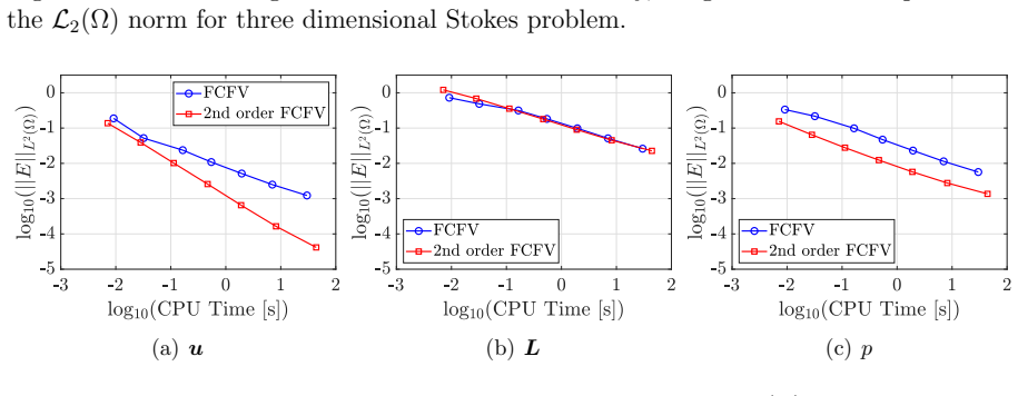
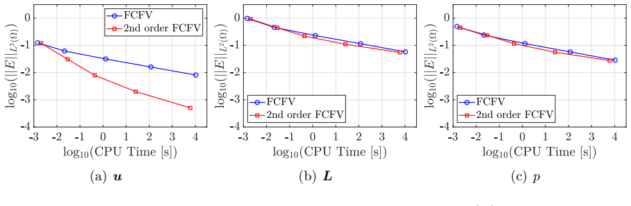
Summary. The paper proposes a second-order face-centred finite volume (FCFV) method for Poisson and Stokes problems. The method uses a mixed formulation with a linear approximation of the solution inside each cell, a constant approximation of its gradient, and a constant approximation of the solution on each cell face. A key ingredient is a projection onto constants in the numerical flux, which the authors state is necessary for second-order accuracy. The solution on the faces is the only globally coupled unknown, so the global system has the same size and sparsity as the previously proposed first-order FCFV method. The paper presents numerical experiments in two and three dimensions showing second-order convergence for the solution/velocity, first-order convergence for the gradient, robustness on distorted and stretched meshes, CPU-time comparisons with the first-order FCFV, two large-scale three-dimensional examples, and an h-adaptive strategy based on the difference between the first- and second-order schemes.
Significance. If the convergence and stability claims are correct, the method is a practically attractive way to obtain second-order accuracy for elliptic and Stokes problems without gradient reconstruction, while keeping a global system of the same size as a first-order method. The numerical evidence is extensive: convergence studies in 2D and 3D, distorted and stretched meshes, CPU-time comparisons, a problem with over five million cells, and an adaptive strategy tested on a complex geometry. The paper is also commendable for reporting timings and for reusing computations between the two schemes in the error indicator. The main weakness is that the central second-order and LBB claims are not proved in the paper but are asserted to be inherited from cited reduced-stabilisation HDG analyses, without verifying that the specific reduced face space used here satisfies the hypotheses of those analyses.
major comments (2)
- [Sections 1 and 2.3, Remark 2] The central claim of second-order convergence is justified only by an inheritance argument: the paper states that the FCFV method 'inherits the convergence properties of HDG' from Oikawa [24,25]. However, the discretisation uses u in V1, q in V0, and the trace unknown in the constant face space V̂0, which is a proper subspace of the trace of V1. The paper does not identify the precise theorems in [24,25], nor does it verify that their hypotheses (in particular on the face approximation space and the role of the projection P0 in the numerical flux) are satisfied by this P1/P0/P0 combination. Because the constant face space is exactly what makes the global system identical in size to the first-order FCFV, the convergence theory must be specific to this reduced face space. The authors should either provide a proof or state and verify the relevant theorem from [24,25] with all hypotheses checked.
- [Section 3, Eq. (41) and Concluding Remarks] For the Stokes problem, the paper asserts that the method 'passes the LBB condition' and presents the discrete problem as the saddle-point system (41), but no inf-sup analysis or proof is given. The well-posedness of the reduced-order Stokes saddle-point problem is load-bearing for the numerical results in Section 5.2 and for the adaptive examples. The authors should provide a discrete inf-sup proof for the constant face space, or precisely identify the result in [25] that covers this case and explain why its assumptions hold here.
minor comments (4)
- [Section 4, Eq. (47)] The relation between the a priori estimate (46) and the desired mesh size (47) is unclear: if ε_e ≤ C h^{1+n_sd/2}, the exponent in (47) should be 1/(1+n_sd/2), not the expression as printed. Please clarify the formula.
- [Section 5.3 and 5.5] There are several typographical errors: 'veloocity gradient' in Section 5.3 and 'randomnly disorted' in Section 5.5. These should be corrected.
- [Section 2.3, Eq. (10)] The operator P0 is introduced as 'the projection operator over the space of constant functions', but it is used on each face individually. It would be clearer to define P0 explicitly as the L2 projection onto constants on each face Γ_e,i, as is done in the proof of Lemma 1.
- [Section 6.1] The claim in the abstract that the method requires a global system with 'identical size and identical number of non-zero elements' is accurate for the global matrix, but the total cost is not identical since the local problems are larger and the assembly time is higher, as noted in Section 6.1. The wording could be qualified to avoid overstatement.
Circularity Check
No circular derivation: the second-order claim rests on an external reduced-stabilisation HDG analysis and on convergence experiments; the only self-citations are minor and non-load-bearing.
full rationale
The claimed second-order convergence is not derived from a fitted parameter or from the paper's own outputs. The formulation is explicit: local problem (8)-(9), projected numerical flux (10), static condensation (21)-(25), and the Stokes analogue (34)-(41). The optimal rates are supported by the external analysis of Oikawa [24,25], invoked in Remark 2 ('the definition of the numerical flux ... follows the rationale of the hybridised DG method with reduced stabilisation. 24'), and by mesh-convergence studies in Sections 5.1-5.2 evaluated against manufactured exact solutions. The tau parameter is tuned in Section 5.4 and then used consistently; it is not a fit constraining the reported convergence rates. The global-system-size identity with the first-order FCFV follows by construction from the constant face trace space and is stated as such, not inferred from data. The error indicator in Section 4 uses an a priori estimate imported from the authors' earlier work [10], but this affects only the adaptive refinement strategy and does not support the central convergence claim. The main caveat is rigor, not circularity: the assertion that the method 'inherits the convergence properties of HDG' is not proved here, so if Oikawa's theorems do not cover the reduced P0 face space, the theoretical basis would be incomplete; the numerical evidence is then the remaining support. That is a correctness risk, not a reduction of the prediction to its inputs.
Assumptions & free parameters
free parameters (1)
- Stabilization parameter tau_e =
tau >= 100 (order of 10^2)
assumptions (4)
- domain assumption The domain is partitioned into conforming simplicial (triangular or tetrahedral) cells with straight faces.
- domain assumption The cited reduced-stabilisation HDG analysis of Oikawa [24, 25] applies to this method, guaranteeing optimal error estimates and LBB stability without further proof in this paper.
- domain assumption The local matrix m_e in Equation (18) is invertible for every cell, including distorted and stretched cells.
- domain assumption The a priori error estimate epsilon_e <= C h^{1+nsd/2} in Equation (46) holds for the FCFV approximation and is used to drive the adaptive process.
Cite this review
Pith. "Pith review of A second-order face-centred finite volume method for elliptic problems." pith.science (2026). https://pith.science/paper/HAHGZ74S
@misc{pith2026190803087,
  author       = {Pith},
  title        = {Pith review of: A second-order face-centred finite volume method for elliptic problems},
  year         = {2026},
  howpublished = {\url{https://pith.science/paper/HAHGZ74S}},
  note         = {Machine review of arXiv:1908.03087}
}
read the original abstract
A second-order face-centred finite volume method (FCFV) is proposed. Contrary to the more popular cell-centred and vertex-centred finite volume (FV) techniques, the proposed method defines the solution on the faces of the mesh (edges in two dimensions). The method is based on a mixed formulation and therefore considers the solution and its gradient as independent unknowns. They are computed solving an element-by-element problem after the solution at the faces is determined. The proposed approach avoids the need of reconstructing the solution gradient, as required by cell-centred and vertex-centred FV methods. This strategy leads to a method that is insensitive to mesh distortion and stretching. The current method is second-order and requires the solution of a global system of equations of identical size and identical number of non-zero elements when compared to the recently proposed first-order FCFV. The formulation is presented for Poisson and Stokes problems. Numerical examples are used to illustrate the approximation properties of the method as well as to demonstrate its potential in three dimensional problems with complex geometries. The integration of a mesh adaptive procedure in the FCFV solution algorithm is also presented.
Figures

Figures from the paper (21 more)








Reference graph
Works this paper leans on
-
[25]
I. Oikawa. Analysis of a reduced-order HDG method for the Stokes equations. Journal of Scientific Computing , 67(2):475–492, 2016
work page 2016
-
[1]
M. Aguirre, A. J. Gil, J. Bonet, and C. H. Lee. An upwind vertex centred finite volume solver for Lagrangian solid dynamics. Journal of Computational Physics, 300:387–422, 2015
work page 2015
-
[2]
T. Barth and M. Ohlberger. Finite volume methods: Foundation and analysis. In Encyclopedia of Computational Mechanics . John Wiley & Sons, Ltd, 2004
work page 2004
-
[3]
J.-C. Chassaing, X. Nogueira, and S. Khelladi. Moving kriging reconstruction for high-order finite volume computation of compressible flows. Computer Methods in Applied Mechanics and Engineering , 253:463–478, 2013
work page 2013
-
[4]
B. Cockburn, B. Dong, and J. Guzm´ an. A superconvergent LDG-hybridizable Galerkin method for second-order elliptic problems. Mathematics of Computation , 77(264):1887–1916, 2008
work page 1916
-
[5]
B. Cockburn and J. Gopalakrishnan. A characterization of hybridized mixed methods for second order elliptic problems. SIAM Journal on Numerical Analysis , 42(1):283– 301, 2004. 28
work page 2004
-
[6]
B. Cockburn and J. Gopalakrishnan. Incompressible finite elements via hybridization. I. The Stokes system in two space dimensions. SIAM Journal on Numerical Analysis , 43(4):1627–1650, 2005
work page 2005
-
[7]
B. Cockburn and J. Gopalakrishnan. New hybridization techniques. GAMM-Mitt., 28(2):154–182, 2005
work page 2005
Show all 34 references
-
[8]
Cockburn, J
B. Cockburn, J. Gopalakrishnan, and R. Lazarov. Unified hybridization of discon- tinuous Galerkin, mixed, and continuous Galerkin methods for second order elliptic problems. SIAM Journal on Numerical Analysis , 47(2):1319–1365, 2009
2009
-
[9]
Cockburn, N
B. Cockburn, N. C. Nguyen, and J. Peraire. A comparison of HDG methods for Stokes flow. Journal of Scientific Computing , 45(1-3):215–237, 2010
2010
-
[10]
D´ ıez and A
P. D´ ıez and A. Huerta. A unified approach to remeshing strategies for finite element h-adaptivity. Computer Methods in Applied Mechanics and Engineering, 176(1-4):215– 229, 1999
1999
-
[11]
Diskin and J
B. Diskin and J. L. Thomas. Comparison of node-centered and cell-centered un- structured finite-volume discretizations: inviscid fluxes. AIAA journal, 49(4):836–854, 2011
2011
-
[12]
Diskin, J
B. Diskin, J. L. Thomas, E. J. Nielsen, H. Nishikawa, and J. A. White. Comparison of node-centered and cell-centered unstructured finite-volume discretizations: viscous fluxes. AIAA journal, 48(7):1326, 2010
2010
-
[13]
Donea and A
J. Donea and A. Huerta. Finite Element Methods for Flow Problems . Finite Element Methods for Flow Problems. John Wiley & Sons, 2003
2003
-
[14]
J. Droniou. Finite volume schemes for diffusion equations: Introduction to and re- view of modern methods. Mathematical Models and Methods in Applied Sciences , 24(08):1575–1619, 2014
2014
-
[15]
Eymard, T
R. Eymard, T. Gallou¨ et, and R. Herbin. Finite volume methods. Handbook of Nu- merical Analysis, 7:713 – 1018, 2000. Solution of Equation in Rn (Part 3), Techniques of Scientific Computing (Part 3)
2000
-
[16]
Giacomini, A
M. Giacomini, A. Karkoulias, R. Sevilla, and A. Huerta. A superconvergent HDG method for Stokes flow with strongly enforced symmetry of the stress tensor. Journal of Scientific Computing , 77(3):1679–1702, 2018
2018
-
[17]
R. J. LeVeque. Finite volume methods for hyperbolic problems . Cambridge Texts in Applied Mathematics. Cambridge University Press, Cambridge, 2002
2002
-
[18]
Montlaur, S
A. Montlaur, S. Fern´ andez-M´ endez, and A. Huerta. Discontinuous Galerkin methods for the Stokes equations using divergence-free approximations. International Journal for Numerical Methods in Fluids , 57(9):1071–1092, 2008. 29
2008
-
[19]
K. W. Morton and T. Sonar. Finite volume methods for hyperbolic conservation laws. Acta Numerica, 16:155–238, 2007
2007
-
[20]
Nguyen, J
N. Nguyen, J. Peraire, and B. Cockburn. A hybridizable discontinuous Galerkin method for Stokes flow. Computer Methods in Applied Mechanics and Engineering , 199(9-12):582–597, 2010
2010
-
[21]
N. C. Nguyen, J. Peraire, and B. Cockburn. An implicit high-order hybridizable discontinuous Galerkin method for linear convection-diffusion equations. Journal of Computational Physics, 228(9):3232–3254, 2009
2009
-
[22]
N. C. Nguyen, J. Peraire, and B. Cockburn. An implicit high-order hybridizable discontinuous Galerkin method for nonlinear convection-diffusion equations. Journal of Computational Physics , 228(23):8841–8855, 2009
2009
-
[23]
N. C. Nguyen, J. Peraire, and B. Cockburn. An implicit high-order hybridizable dis- continuous Galerkin method for the incompressible Navier-Stokes equations. Journal of Computational Physics , 230(4):1147–1170, 2011
2011
-
[24]
I. Oikawa. A hybridized discontinuous Galerkin method with reduced stabilization. Journal of Scientific Computing , 65(1):327–340, 2015
2015
-
[26]
Qiu and K
W. Qiu and K. Shi. A superconvergent HDG method for the incompressible Navier– Stokes equations on general polyhedral meshes. IMA Journal of Numerical Analysis , 36(4):1943–1967, 2016
1943
-
[27]
R. Sevilla. HDG-NEFEM for two dimensional linear elasticity. Computers & Struc- tures, 220:69–80, 2019
2019
-
[28]
Sevilla, M
R. Sevilla, M. Giacomini, and A. Huerta. A face-centred finite volume method for second-order elliptic problems. International Journal for Numerical Methods in En- gineering, 115(8):986–1014, 2018
2018
-
[29]
Sevilla, M
R. Sevilla, M. Giacomini, and A. Huerta. A locking-free face-centred finite volume (FCFV) method for linear elastostatics. Computers & Structures , 212:43–57, 2019
2019
-
[30]
Sevilla, M
R. Sevilla, M. Giacomini, A. Karkoulias, and A. Huerta. A superconvergent hybridis- able discontinuous Galerkin method for linear elasticity. International Journal for Numerical Methods in Engineering , 116(2):91–116, 2018
2018
-
[31]
Sevilla and A
R. Sevilla and A. Huerta. Tutorial on Hybridizable Discontinuous Galerkin (HDG) for second-order elliptic problems. In J. Schr¨ oder and P. Wriggers, editors, Advanced Finite Element Technologies, volume 566 ofCISM International Centre for Mechanical Sciences, pages 105–129. S...
2016
-
[32]
Sevilla and A
R. Sevilla and A. Huerta. HDG-NEFEM with degree adaptivity for Stokes flows. Journal of Scientific Computing , 77(3):1953–1980, 2018
1953
-
[33]
E. F. Toro. Riemann solvers and numerical methods for fluid dynamics . Springer- Verlag, Berlin, third edition, 2009. A practical introduction
2009
-
[34]
X. Yang, C. Liu, Y. Li, F. Marchesoni, P. H¨ anggi, and H. Zhang. Hydrodynamic and entropic effects on colloidal diffusion in corrugated channels. Proceedings of the National Academy of Sciences , 114(36):9564–9569, 2017. 31
2017
Reviewed August 14, 2026 · model on record in the stance chip above.
Discussion (0). Continue with ORCID to comment.