Turbulence driven by stellar jets, the possibility and the efficiency

Mohsen Abgharian-Afoushteh; Somayeh Sheikhnezami

REVIEW 4 major objections 4 minor 42 references

Turbulence driven by stellar jets, the possibility and the efficiency

T0 review · 4 major / 4 minor · reviewed 2026-08-14 · deepseek-v4-flash

Challenge this review Re-run · record.json Download PDF Read on arXiv ↗ Review JSON

Pith's one-line read Stellar jets can transfer turbulence to neighboring regions but are not sufficient drivers of the large-scale supersonic turbulence in molecular clouds, these simulations conclude.

desk verdict A competent but incremental parameter scan of jet-driven turbulence; the qualitative conclusion is probably right, but the main diagnostic does not separate the jet beam from actual turbulent fluctuations. read the letter →

arxiv 1908.03225 v1 pith:FS4XSHD6 submitted 2019-08-08 astro-ph.HE astro-ph.GA

Somayeh Sheikhnezami , Mohsen Abgharian-Afoushteh This is my paper · ORCID

classification astro-ph.HEastro-ph.GA

keywords stellarjetsmolecularcloudssupersonicturbulenceprotostellaroutflowsmagnetohydrodynamicsnumericalsimulationvelocityprobabilitydensityfunctionstarformation

verification ladder T0 review T1 audit T2 compute T3 formal

The pith

A machine-rendered reading of the paper's core claim, the machinery that carries it, and where it could break.

The reading

This paper asks whether the jets launched by young stars can be the engine of the supersonic turbulence seen in molecular clouds. The authors run a battery of two- and three-dimensional hydrodynamics and magnetohydrodynamics simulations that vary the jet's Mach number, its velocity structure, the background magnetic field, the cloud environment, and the number of interacting jets. They find that jets do inject random, turbulent motions into the surrounding gas, and that the injection is stronger for faster jets, rotating jets, magnetized environments, clumpy environments, and multiple interacting jets. However, most of the entrained gas stays subsonic or transonic, and once the jet stops driving, the supersonic fluctuations decay quickly. The conclusion is that jets are effective local stirring agents but cannot sustain the large-scale supersonic turbulence of molecular clouds, which matters because that turbulence is thought to control how and where stars form.

What carries the argument

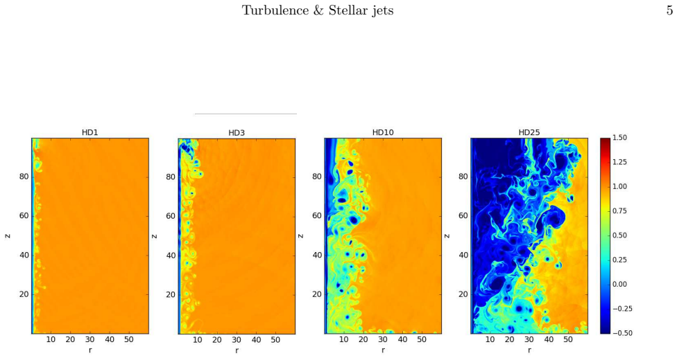
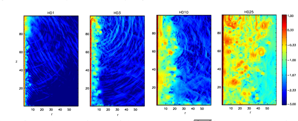
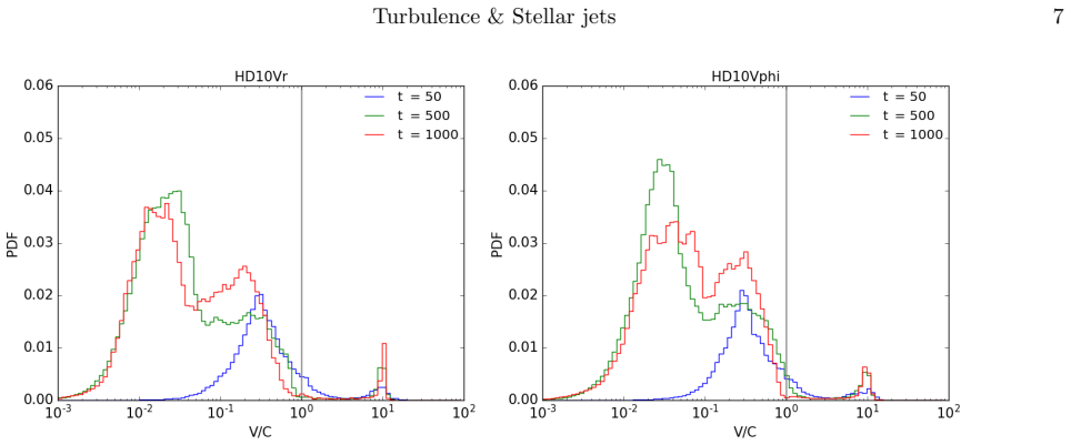
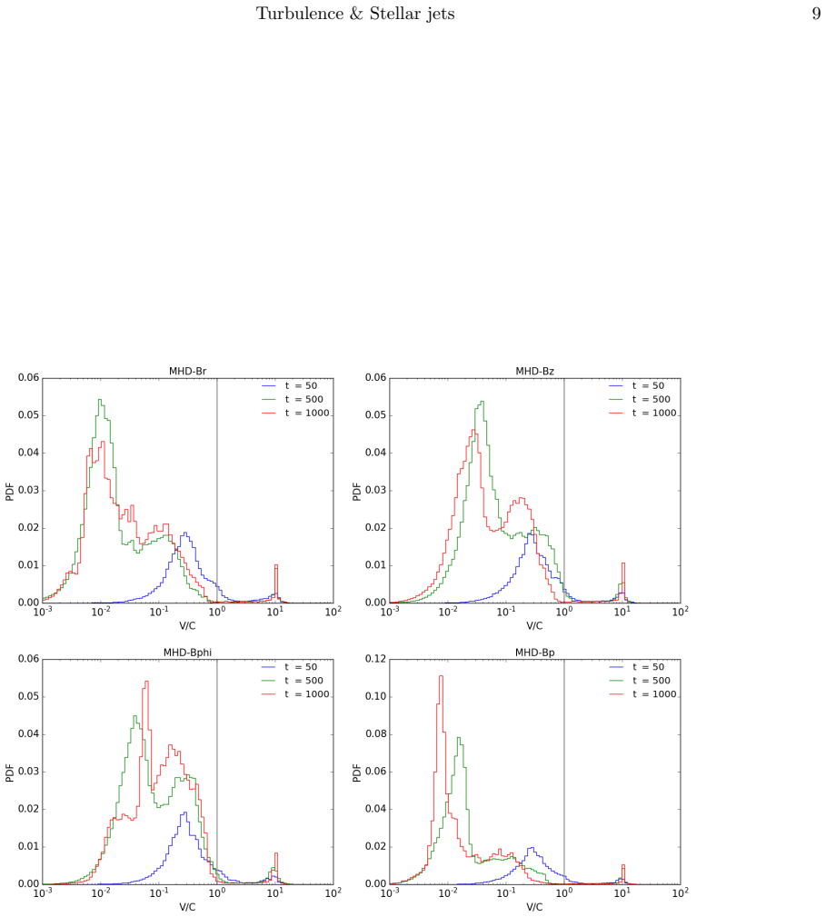
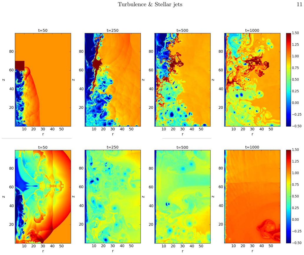
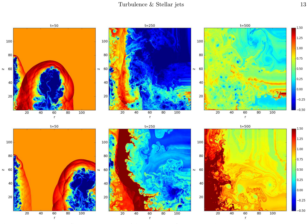
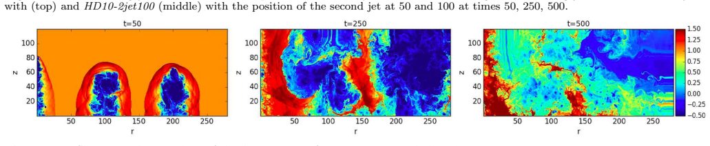
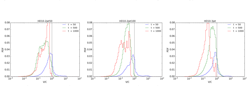
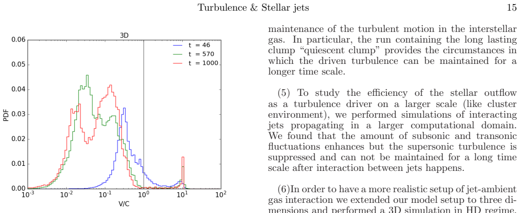
The central measurement is the velocity probability density function (PDF), defined by binning the poloidal velocity $v_p = \sqrt{v_r^2 + v_z^2}$ over all cells excited by the jet and normalizing by the total number of cells. Comparing the PDF with the local sound speed allows the authors to split the entrained gas into subsonic and supersonic populations and to track how the high-velocity tail decays after the jet engine is switched off. This PDF sits at the center of a deliberately broad parameter study: hydrodynamic and ideal-magnetohydrodynamic runs on a $60 \times 100$ jet-radius grid, with Mach numbers 1, 3, 10 and 25; runs with added radial or rotational jet velocity; runs with radial, vertical, toroidal, and poloidal background fields; runs with a quiescent or explosive dense clump in the ambient gas; runs with two or three interacting jets; and one 3D counterpart of the reference run. The comparison set is what lets the paper claim that the efficiency, not just the possibility, of jet-driven turbulence depends on these parameters.

What would settle it

A numerical experiment that switches a jet off at late time and measures the mass fraction of supersonic gas afterward: the paper reports that no supersonic features survive after switch-off, so any run that sustains a significant supersonic fraction for many crossing times after the jet dies would refute the claim. Observationally, mapping a star-forming region where outflows have recently ceased and finding cloud-scale supersonic line widths uncorrelated with outflow power would likewise contradict the insufficiency conclusion.

Watch

Extended reading notes

Core claim

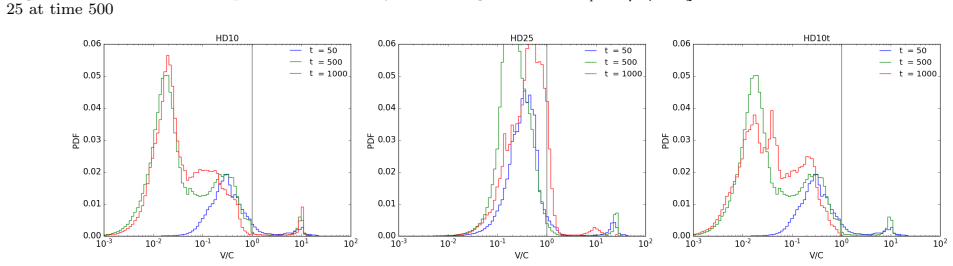
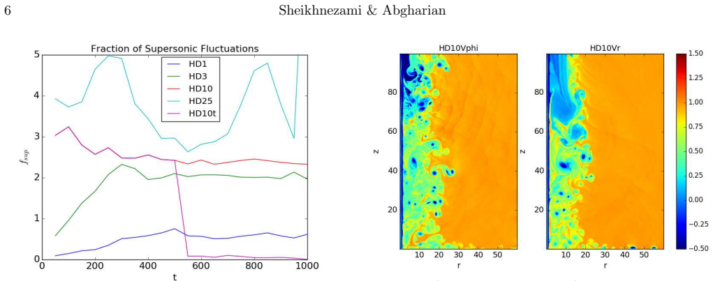
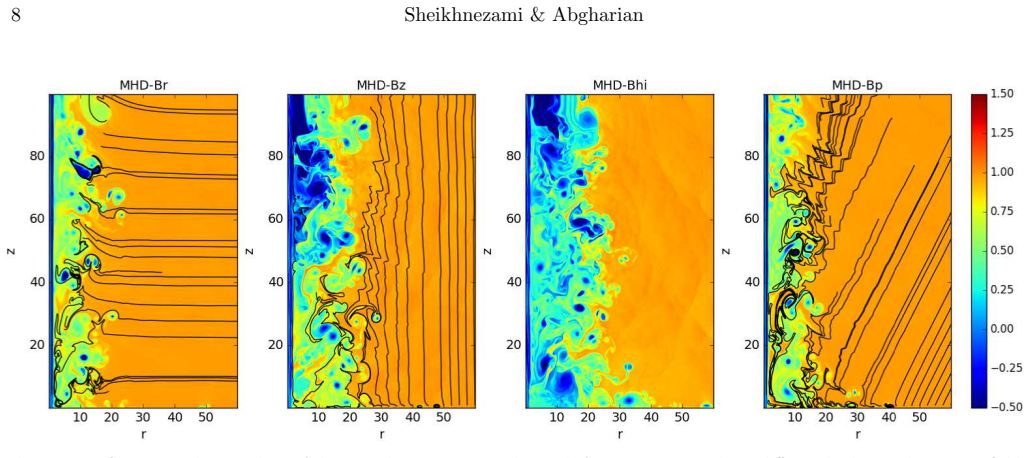
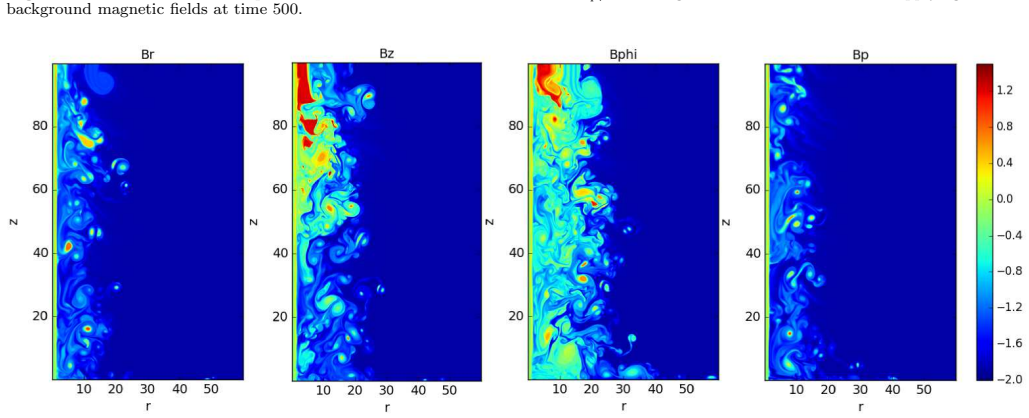
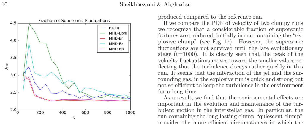
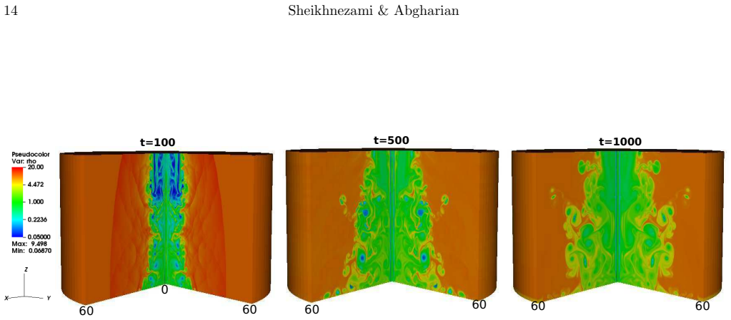
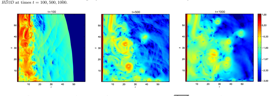
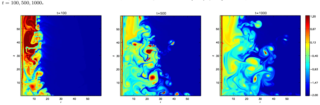
On the paper's own terms, the central discovery is a confirmation with expanded parameter coverage: protostellar jets transfer turbulence to their immediate neighborhood, but they are not sufficient drivers of large-scale supersonic turbulence in molecular clouds. The evidence is the velocity probability density function of the entrained gas: in every run the bulk of the excited motions lies at subsonic velocities, with only a small fraction supersonic, and that fraction decreases with time. A transient-jet run shows that when the driving stops, the supersonic part disappears almost immediately. The efficiency of the local driving does vary: higher Mach number, jet rotation, a toroidal background magnetic field, a clumpy ambient medium, and interacting jets all raise the amount and longevity of the fluctuations, and a 3D run produces more and faster entrained gas than the axisymmetric runs, though the paper attributes part of that enhancement to the lower resolution and higher numerical diffusivity of the 3D setup.

Load-bearing premise

The load-bearing premise is that a simulation box of about $10^4$ AU and simulated times of up to a few thousand time units (roughly $10^5$ to $10^6$ yr) captures the processes that decide whether jets can drive cloud-scale turbulence, even though the cloud itself is orders of magnitude larger and longer-lived.

Editorial extensions

If this is right

In the immediate vicinity of a protostellar outflow, jets can keep the gas stirred with subsonic and transonic velocity fluctuations for as long as the jet keeps running.
A single transient protostellar jet cannot maintain supersonic turbulence: once the jet is switched off, the supersonic fraction of the entrained gas drops away, so outflow feedback must be continuous or constantly replenished by new outflows to matter.
The most powerful outflows, with higher Mach numbers, are the ones most likely to leave a lasting turbulent imprint on their surroundings, since their pdfs stay broader and their supersonic fractions survive longer.
Outflow interactions in clustered star formation mainly add transonic and subsonic fluctuations; after jets collide, supersonic motions are suppressed, so cluster-scale multiple outflows do not by themselves solve the cloud-scale supersonic driving problem.
In magnetized clouds, the toroidal field geometry is the one that most increases the entrained gas energy and the supersonic fraction, meaning the orientation of the background field relative to the outflow matters for feedback efficiency.

Reading between the lines

Editorial extensions of the paper, not claims the author makes directly.

Beyond the paper, if jets are only local drivers, then the global supersonic line widths of molecular clouds have to be sustained by processes the small box cannot see, such as large-scale gravitational contraction, converging flows, or supernova remnants, and jet feedback would set the local velocity dispersion near outflow cavities rather than the cloud's global turbulence.
Beyond the paper, a testable extension would be a resolution-convergence study: the paper's 3D run mixes the physical growth of non-axisymmetric shear modes with numerical diffusivity from a lower resolution, so a matched-resolution 2D versus 3D comparison would isolate how much of the extra 3D fluctuations is real.
Beyond the paper, the interacting-jet simulations suggest a saturation effect: adding more jets raises the transonic gas but suppresses supersonic tails, so one could predict that in a dense cluster the outflow-driven velocity dispersion approaches a ceiling set by jet separation and cooling, a relation observable as a flattening of outflow power versus local line width.

Share X Bluesky LinkedIn Reddit HN

Signed reviews

No signed human review yet.

Editorial analysis

A structured set of objections, weighed in public.

Desk editor's note, referee report, and a circularity audit.

Desk Editor's Note

read the letter

Plain English: this paper is a numerical case study of protostellar jets driving turbulence. The genuinely useful part is the breadth: Mach number, rotation, magnetic field geometry, clumpy environment, interacting jets, and one 3D run, all with the same code and setup. That is more coverage than Banerjee et al. 2007 or Cunningham et al. 2009. The authors are honest that they are confirming prior conclusions, not overturning them. The runs look like standard PLUTO, the setup is sensible, and the qualitative behavior (bow shock, shear, entrainment, decay after switching off) matches expectation. I believe them when they say jets drive local, mostly subsonic motions and are not large-scale supersonic drivers.

But I would not trust the efficiency rankings yet. The quantitative measure is the velocity PDF over every cell with nonzero velocity. That includes the continuously injected jet beam, whose vp is supersonic by construction. The transient run is the giveaway: after the jet is switched off, the supersonic part of the PDF disappears within a few sound-crossing times. That is the beam vanishing, not a turbulence cascade decaying. So the claim that higher Mach number, rotation, toroidal fields, clumps, interacting jets, or 3D geometry increase 'turbulence' is really about the total velocity distribution, with beam and shocked gas mixed in. A proper analysis would mask the beam or Reynolds-decompose and look at the velocity dispersion of the ambient gas, or use a structure function or power spectrum. Without that, the efficiency results are suggestive, not established.

There are lesser issues. No resolution study, so numerical diffusivity could be doing some of the work; the 3D run is actually lower resolution and the authors admit it has higher numerical viscosity, which muddies the 3D comparison. The box is ~10^4 AU, so the claim about 'large-scale' turbulence in molecular clouds is an extrapolation, not something the simulation directly tests. The authors do flag the box-size limitation in Section 3, which is to their credit. The citation pattern looks fine: Banerjee et al. and Cunningham et al. are properly credited, and the paper explicitly frames itself as confirmation. No obvious circularity.

Bottom line: the qualitative conclusion is probably correct and consistent with the literature. The quantitative efficiency story is not yet supported. This is a decent candidate for a revised paper, not a desk reject, but it needs a better turbulence diagnostic and at least one convergence run before I would rely on it.

Referee Report

4 major / 4 minor

Summary. The manuscript reports a parameter study of two-dimensional axisymmetric and one three-dimensional hydrodynamic/magnetohydrodynamic simulations of protostellar jets interacting with a uniform or clumpy ambient medium, using the PLUTO 4.2 code. The models vary the jet Mach number (1, 3, 10, 25), the jet velocity field (radial and rotational components), the background magnetic field geometry, the presence of dense clumps, and the number of interacting jets. The principal diagnostic is the probability density function of the poloidal velocity magnitude (Eq. 5), from which the fraction of supersonic gas and its time evolution are measured. The central conclusion is that stellar jets can transfer turbulent motions to their immediate surroundings, with higher efficiency for higher jet Mach number, jet rotation, toroidal background magnetic fields, clumpy environments, jet-jet interactions, and three-dimensional geometry, but that jets are not sufficient drivers of large-scale supersonic turbulence in molecular clouds.

Significance. The question addressed is important for star-formation feedback, and the manuscript usefully expands the parameter space covered by earlier studies such as Banerjee et al. (2007). Its strengths include a systematic set of models in a well-tested code, a transient-jet experiment designed to measure the decay of the induced motions, and explicit admissions of the limitations imposed by the box size and by the lower resolution of the 3D run. If the central result is accepted, it strengthens the emerging picture that protostellar outflows are local turbulence drivers rather than cloud-scale supersonic drivers. However, because the velocity PDF used as the turbulence measure includes the coherent jet beam and no decomposition into mean and fluctuating components is made, the quantitative efficiency rankings are not yet established by the presented analysis; the paper's significance therefore depends on a re-analysis described below.

major comments (4)

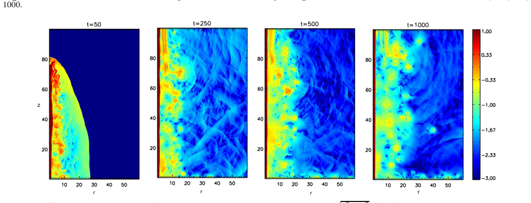
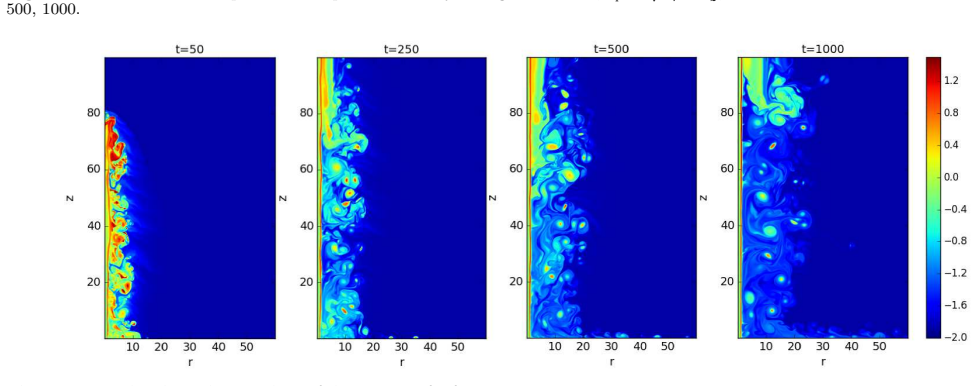
[2.4, 3, Figs. 6, 7, 15, 20, 24] Equation (5) defines the velocity PDF using vp = sqrt(vr^2+vz^2) over all cells with nonzero velocity, so it counts the ordered, continuously injected jet beam together with any turbulent fluctuations. For the supersonic runs (M=10 and 25), cells inside the jet beam have vp > c_s by construction, so the 'supersonic fraction' plotted in Figures 7, 15, 20, and 24 is contaminated by the beam's coherent kinetic energy. The transient run HD10t (Figure 6) illustrates this: once the jet is switched off, the supersonic component disappears within a few hundred code units, which is exactly what one expects when the beam is removed, not necessarily evidence about the decay of a turbulent cascade. The efficiency rankings listed in the abstract and Section 4 are therefore rankings of the total velocity distribution, not of turbulence. I request a Reynolds decomposition or a masking of the jet-beam region (for example, cells with r < r_j and/or cells connected to the injection boundary) and the PDF of the fluctuating component, together with a velocity power spectrum, before the central claim of 'transferring turbulence' can be assessed quantitatively.
[3, 3.1-3.5] The term 'turbulence' is used for what the velocity PDF and visual inspection of maps show, but a one-point PDF of the total velocity does not establish a turbulent cascade or distinguish random motions from coherent shear, and it cannot provide a scale-dependent measure of driving efficiency. No velocity power spectrum, structure function, or vorticity map is presented anywhere in the paper. The qualitative statements about 'more fluctuations and random motions' in Sections 3.1-3.5 are therefore not backed by a quantitative turbulence metric. I recommend adding at least one scale-resolved statistic (for example, a kinetic-energy power spectrum, a longitudinal structure function, or a vorticity map) to justify the term 'turbulence' and the efficiency rankings.
[2.2, 3.5] No resolution or convergence study is reported for the axisymmetric runs, and the single 3D run uses a lower resolution than the 2D reference run (Section 3.5). The authors themselves note that the lower resolution implies higher numerical diffusivity and numerical heating that increase the entropy and the amount of fluctuations in HD3D. Since the paper's quantitative conclusions depend on PDF tails, supersonic fractions, and their decay times, a convergence check is load-bearing; without it, one cannot separate physical turbulence driving from numerical diffusion, and the 3D-versus-2D comparison is ambiguous. I ask for at least one higher-resolution 3D run (or two resolutions of the reference run with the same solver and domain) and a brief comparison of the PDF and supersonic fraction as a function of resolution.
[3, 4] The concluding statement that jets are 'not sufficient drivers of the large-scale supersonic turbulence in molecular clouds' goes beyond the simulated domain, which is 60 x 100 r_j (about 10^4 AU) and which the authors themselves describe as smaller than the scale of interest, with the ambient gas still affected by jet propagation at the end of the runs (Section 3). The simulations contain no cloud-scale driving or large-scale velocity structure, so they can only constrain turbulence within a small star-forming core environment, not the maintenance of cloud-scale supersonic turbulence. The abstract and Section 4 should be reframed to state the negative result for the box scale, or supplemented with a quantitative argument connecting the box-size results to cloud scales (for example, comparing the turbulent energy injection rate with the dissipation rate on cloud scales).

minor comments (4)

[3.3, Table 1] Section 3.3 refers to runs HD-M10cl and HD-M10pcl, while Table 1 lists the same runs as HD-Qcl and HD-Ecl; please make the run labels consistent throughout the manuscript.
[2.3, 3.2, 4] There are several typographical errors that should be corrected: 'grcm' for 'g cm^-3', 'solenodality' for 'solenoidality', 'magnetite' for 'magnetic' in Section 3.2, and 'peresented' and 'studeid' in Section 4.
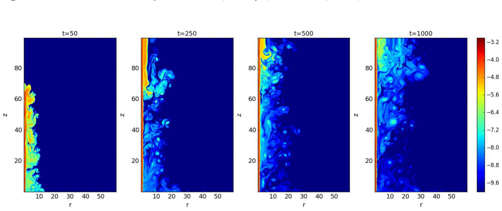
[3, Figs. 3, 13, 23] The 'entropy' shown in Figures 3, 13, and 23 is never defined in Section 2; please specify the entropy diagnostic (for example, p/rho^gamma or a normalized version) so that the reader can interpret the maps.
[3.5] The actual grid resolution of the 3D run HD3D is not reported in the text or in Table 1; since the authors state that the 3D run uses a lower resolution, the numerical setup is incomplete without the specific number of cells.

Circularity Check

0 steps flagged · score 0.0 of 10

No significant circularity found; the conclusions are drawn from simulations with hand-chosen inputs and compared against no fitted target.

full rationale

The paper's central claims are derived from PLUTO simulations with parameters chosen as a case study rather than fitted to reproduce any target outcome. The velocity PDF defined in Eq. 5 is a diagnostic applied to simulation output, not a quantity that the simulations were tuned to match. The transient-jet run HD10t is used as a physical control to show decay of supersonic features after driving stops, which is an independent behavioral test rather than a circular construct. The negative claim about large-scale supersonic turbulence is explicitly qualified by the box-size limitation noted in Section 3, and it is presented as confirmation of earlier independent work rather than as a consequence of a self-citation. The paper's self-citations concern jet-launching simulations and do not carry the load of the turbulence-efficiency argument. The skeptic's concern that the velocity PDF conflates the coherent jet beam with turbulent fluctuations is a substantive validity critique of the diagnostic, not evidence that a prediction is equivalent to an input by construction. No fitted parameter is renamed as a prediction, no uniqueness theorem is imported from the authors' prior work, and no ansatz is smuggled in via citation. Therefore the circularity score is 0.

Assumptions & free parameters 5 free parameters · 6 assumptions · 0 invented entities

The paper is a numerical experiment; the listed parameters are hand-chosen initial conditions for the case study, not constants fitted to observations. No invented entities are introduced. The core axioms are the ideal MHD/HD equations, a polytropic EOS with gamma=5/3 and no cooling, pressure equilibrium between jet and ambient gas, and axisymmetry for the 2D runs.

free parameters (5)

Density contrast delta = rho_j/rho_a = 0.1 (chosen uniformly across runs)
Jet/ambient density ratio set to 0.1 in all runs (Table 1); affects entrainment and turbulence generation.
Jet Mach number = 1, 3, 10, 25
Central parameter of study; higher M increases excited gas and PDF peak velocities; no external calibration.
Background magnetic field strengths = B_r=0.001, B_z=0.002, B_phi=0.001 in code units
Field geometries in MHD runs (Table 1); chosen ad hoc to compare radial, vertical, toroidal, and poloidal configurations.
Radial and rotational jet velocity components = v_r=0.01, v_phi=0.01 (code units)
Used in HD10Vr and HD10Vphi to study the effect of velocity field on jet-ambient interaction.
Clump properties = Not quantified in text
Quiescent clump (overdense, pressure equilibrium) and explosive clump (overdense, overpressured) defined qualitatively in Section 3.3; no numerical values given.

assumptions (6)

domain assumption Ideal MHD/HD equations are the correct description; no resistivity or explicit diffusion in the induction equation.
Equations (1)-(4); the paper states that including heating/cooling and non-ideal MHD is deferred to future work.
domain assumption Polytropic equation of state with gamma=5/3 and no heating/cooling.
Section 2.1: 'The gas pressure follows a polytropic equation of state P = (gamma-1)u with gamma = 5/3'; cooling is not included.
domain assumption Jet is initially in pressure equilibrium with the ambient gas.
Section 2.1 states 'the jet area has a lower density but is in pressure equilibrium with the ambient gas'; used to justify that interaction is via shear instabilities.
ad hoc to paper Axisymmetry in the 2D runs is representative of the jet-ambient interaction.
All runs except HD3D are axisymmetric; Section 3.5 acknowledges shear instabilities in azimuthal direction are not captured in 2D. This is load-bearing for the 2D parameter ranking.
ad hoc to paper The small computational box (60 x 100 r_j, about 10^4 AU) is representative of molecular-cloud turbulence driving scales.
Section 3 notes the box size is smaller than cloud scales, yet conclusions about 'large-scale' supersonic turbulence are drawn.
domain assumption Continuously powered jet injection at the lower boundary represents a formed jet.
Section 2.2: 'in all runs presented here the injected jet is continuously powered'; no self-consistent launching is modeled.

how reviews work

0 comments

Cite this review

Pith. "Pith review of Turbulence driven by stellar jets, the possibility and the efficiency." pith.science (2026). https://pith.science/paper/FS4XSHD6

@misc{pith2026190803225,
  author       = {Pith},
  title        = {Pith review of: Turbulence driven by stellar jets, the possibility and the efficiency},
  year         = {2026},
  howpublished = {\url{https://pith.science/paper/FS4XSHD6}},
  note         = {Machine review of arXiv:1908.03225}
}

read the original abstract

We investigate the feedback of the stellar jets on the surrounding interstellar gas based on 2D and 3D simulations applying HD and MHD module of PLUTO 4.2 code. The main question we address is whether the stellar jet can be considered as a turbulence driver into the interstellar gas. In addition, we investigate the most effective circumstances in which the driven turbulence is larger and can survive for a longer time scale in the ambient gas. We present a case study of different parameters runs including the jet Mach number, the initial jet velocity field and the background magnetic field geometries and the interacting jets. Also, we study the environmental effects on the jet-gas interaction by considering the non-homogeneous surrounding gas containing the clumps in the model setup. Among different setups, we find that for (1) a higher jet Mach number, (2) a rotating jet, 16 pages(3) a jet propagating in a magnetized environment, (4)a jet propagating in a non-homogeneous environment, and (5) the interacting jets more fluctuations and random motions are produced in the entrained gas which can survive for a longer time scale. In addition, we perform the 3D simulations of jet-ambient gas interaction and we find that the amount of (subsonic-supersonic) fluctuations increases compared to the axisymmetric run and the entrained gas gains higher velocities in a 3D run. In total, we confirm the previous finding that the stellar jets can transfer the turbulence on neighboring regions and are not sufficient drivers of the large-scale supersonic turbulence in molecular clouds.

Figures

Figures reproduced from arXiv: 1908.03225 by the authors.

**Figure 1.** Reference run. Shown are the snapshots of the mass density in Logarithm scale for reference run HD10 at times 50, 250, 500, 1000. z r r r r [PITH_FULL_IMAGE:figures/full_fig_p004_1.png] view at source ↗

**Figure 2.** Shown are the snapshots of the poloidal velocity in Logarithm scale, vp = p v 2 r + v 2 z , for reference run HD10 at times 50 ,250, 500, 1000 [PITH_FULL_IMAGE:figures/full_fig_p004_2.png] view at source ↗

**Figure 3.** Displayed are the snapshots of the entropy of reference run HD10 at times 50, 250, 500, 1000 [PITH_FULL_IMAGE:figures/full_fig_p004_3.png] view at source ↗

Figures from the paper (20 more)

**Figure 4.** Figure 4: Shown are the snapshots of the mass density in Logarithm scale for runs with Mach numbers of 1, 3, 10 and 25 at time 500. z r r r r [PITH_FULL_IMAGE:figures/full_fig_p005_4.png]

**Figure 5.** Figure 5: Shown are the snapshots of the velocity field in Logarithm scale vp = p v 2 r + v 2 z for runs with Mach numbers of 1, 3, 10 and 25 at time 500 [PITH_FULL_IMAGE:figures/full_fig_p005_5.png]

**Figure 6.** Figure 6: Shown are the plots of the probability density function of velocity for run HD10,HD25 and HD10t at times 50, 500, 1000. Here C denotes to the local sound speed of the gas. The vertical line shows the transonic velocity and distinguishes between the subsonic and the sup…

**Figure 8.** Figure 8: Shown are the snapshots of the mass density in Logarithm scale for runs HD10Vr, HD10Vphi including radial and rotational jet velocity, respectively. 8. Compared to the reference run including the jet radial velocity or the jet rotation increases the size of the entr…

**Figure 9.** Figure 9: Shown are the PDF of velocity for runs HD10Vr, HD10Vphi, at times t = 50, t = 500, t = 1000 [PITH_FULL_IMAGE:figures/full_fig_p007_9.png]

**Figure 10.** Figure 10: Centrifugal force. Shown are the snapshots of the centrifugal force for run HD10Vphi including jet rotational velocity. the mass density distribution of all MHD runs [PITH_FULL_IMAGE:figures/full_fig_p007_10.png]

**Figure 11.** Figure 11: Shown are the snapshots of the mass density in Logarithm scale for MHD runs applying different background magnetic fields at time 500. The field lines are shown in black. r z r r r [PITH_FULL_IMAGE:figures/full_fig_p008_11.png]

**Figure 12.** Figure 12: Shown are the snapshots of the Alfven Mach number MA = vp/vA in Logarithm scale for MHD runs applying different background magnetic fields at time 500 [PITH_FULL_IMAGE:figures/full_fig_p008_12.png]

**Figure 13.** Figure 13: Shown are the snapshots of the entropy of gas in Logarithm scale for MHD run applying different background magnetic fields at time 500 [PITH_FULL_IMAGE:figures/full_fig_p008_13.png]

**Figure 14.** Figure 14: Shown are the Probability density functions of velocity for MHD runs at different times [PITH_FULL_IMAGE:figures/full_fig_p009_14.png]

**Figure 15.** Figure 15: Shown is a comparison of the evolution of the supersonic features with respect to all gas materials for the MHD runs and the reference run. during the time. However, it is seen that in a run with the toroidal field, the fraction of the supersonic features in the ambi…

**Figure 16.** Figure 16: Shown are the snapshots of the mass density for run HD-Qcl (top) and run HD-Ecl at times 50,250, 500, and 1000 [PITH_FULL_IMAGE:figures/full_fig_p011_16.png]

**Figure 17.** Figure 17: Shown are the Probability density functions of velocity for runs, HD-Qcl and HD-Ecl at different times [PITH_FULL_IMAGE:figures/full_fig_p011_17.png]

**Figure 18.** Figure 18: Interacting jets. Shown are the snapshots of the density mass of runs including the interacting jets, i.e., run HD10-2jet50 with (top) and HD10-2jet100 (middle) with the position of the second jet at 50 and 100 at times 50, 250, 500 [PITH_FULL_IMAGE:figures/full_fig_…

**Figure 19.** Figure 19: Shown are the snapshots of the density mass of run HD10-3jet including three interacting jets at times 50, 250, 500 [PITH_FULL_IMAGE:figures/full_fig_p013_19.png]

**Figure 20.** Figure 20: Shown are the plots of the probability Density Function of velocity for run HD10-2jet50, HD10-2jet100 and HD10-3jet including interacting jets at times 50, 500, 1000 [PITH_FULL_IMAGE:figures/full_fig_p013_20.png]

**Figure 21.** Figure 21: 3D evolution of jet-ambient gas system. Shown are the cuts of the mass density distribution in three dimensions for run HD3D at times t = 100, 500, 1000 [PITH_FULL_IMAGE:figures/full_fig_p014_21.png]

**Figure 22.** Figure 22: Shown are 2D slices of the velocity field in Logarit [PITH_FULL_IMAGE:figures/full_fig_p014_22.png]

**Figure 23.** Figure 23: Shown are 2D slices of the entropy in Logarithm sca [PITH_FULL_IMAGE:figures/full_fig_p014_23.png]

**Figure 24.** Figure 24: Shown are the plots of the probability Density Function of velocity for run HD3D at times 50, 500, 1000. stellar jets. We found a clear correlation between the excited gas and the jet Mach number. By increasing the jet Mach number a faster continues jet is injected i…

Discussion (0). Continue with ORCID to comment.

Reference graph

Works this paper leans on

42 extracted references · 33 canonical work pages

[1]

1996, ApJ, 473, 921

Bally, J., Devine, D., & Alten, V. 1996, ApJ, 473, 921

work page 1996
[2]

& Reipurth, B

Bally, J. & Reipurth, B. 2003, AJ, 126, 893

work page 2003
[3]

S., & Fendt, C

Banerjee, R., Klessen, R. S., & Fendt, C. 2007, ApJ, 668, 1028

work page 2007
[4]

C., Blandford, R

Begelman, M. C., Blandford, R. D., & Rees, M. J. 1984, Reviews of Modern Physics, 56, 255

1984
[5]

Blandford, R. D. & Payne, D. G. 1982, MNRAS, 199, 883

1982
[6]

2017, A&A, 601, A9 0

Brauer, R., W olf, S., Reissl, S., & Ober, F. 2017, A&A, 601, A9 0

work page 2017
[7]

J., Frank, A., & Blackman, E

Carroll, J. J., Frank, A., & Blackman, E. G. 2010, ApJ, 722, 14 5

work page 2010
[8]

Quillen, A. C. 2009, ApJ, 695, 1376

work page 2009

Show all 42 references

[9]

2010, A&A, 512, A54

Asplund, M. 2010, A&A, 512, A54

2010
[10]

& Keppens, R

Casse, F. & Keppens, R. 2002, ApJ, 581, 988

2002
[11]

Crutcher, R. M. 1999, ApJ, 520, 706

1999
[12]

M., Troland, T

Crutcher, R. M., Troland, T. H., Lazareﬀ, B., Paubert, G., & Kaz` es, I. 1999, ApJ, 514, L121

1999
[13]

Quillen, A. C. 2009, ApJ, 692, 816

2009
[14]

2000, ApJ, 530, 923 16 Sheikhnezami & Abgharian

Delamarter, G., Frank, A., & Hartmann, L. 2000, ApJ, 530, 923 16 Sheikhnezami & Abgharian

2000
[15]

1997, A&A, 319, 340 G´ omez, J

Ferreira, J. 1997, A&A, 319, 340 G´ omez, J. L., Lobanov, A. P., Bruni, G., Kovalev, Y. Y.,

1997
[16]

V., Anderson, J

Sokolovsky, K. V., Anderson, J. M., Galindo, P., Kardashev, N. S., & Lisakov, M. M. 2016, ApJ, 817, 96

2016
[17]

E., Klein, R

Hansen, C. E., Klein, R. I., McKee, C. F., & Fisher, R. T. 2012, ApJ, 747, 22

2012
[18]

A., Miller, M

Hughes, P. A., Miller, M. A., & Duncan, G. C. 2002, ApJ, 572, 713

2002
[19]

R., Mac Low, M.-M., & Bryan, G

Joung, M. R., Mac Low, M.-M., & Bryan, G. L. 2009, ApJ, 704, 137

2009
[20]

2013, Plasma Physics and Controlled Fusion, 55, 124038

Keppens, R., Porth, O., Monceau-Baroux, R., & W alg, S. 2013, Plasma Physics and Controlled Fusion, 55, 124038

2013
[21]

Knee, L. B. G. & Sandell, G. 2000, A&A, 361, 671

2000
[22]

Krumholz, M. R. & Tan, J. C. 2007, ApJ, 654, 304

2007
[23]

& Nakamura, F

Li, Z.-Y. & Nakamura, F. 2006, ApJ, 640, L187 Mac Low, M.-M. 2000, in ESA Special Publication, Vol. 445, St ar Formation from the Small to the Large Scale, ed. F. Favata, A. Kaas, & A. Wilson, 457 Mac Low, M.-M. & Klessen, R. S. 2004, Reviews of Modern Physics, 76, 125

2006
[24]

R., & Ryle, W

Sigua, L., Miller, H. R., & Ryle, W. T. 2008, Nature, 452, 966

2008
[25]

McKee, C. F. & Ostriker, E. C. 2007, ARA&A, 45, 565

2007
[26]

2007, ApJS, 170, 228

Mignone, A., Bodo, G., Massaglia, S., Matsakos, T., Tesilea nu, O., Zanni, C., & Ferrari, A. 2007, ApJS, 170, 228

2007
[27]

2013, MNRAS, 436, 1102

Mignone, A., Striani, E., Tavani, M., & Ferrari, A. 2013, MNRAS, 436, 1102

2013
[28]

2012, ApJS, 198, 7

Mignone, A., Zanni, C., Tzeferacos, P., van Straalen, B., Co lella, P., & Bodo, G. 2012, ApJS, 198, 7

2012
[29]

C., Stone, J

Ostriker, E. C., Stone, J. M., & Gammie, C. F. 2001, ApJ, 546, 980

2001
[30]

2013, MNRAS, 429, 2482

Porth, O. 2013, MNRAS, 429, 2482

2013
[31]

Pudritz, R. E. & Norman, C. A. 1983, ApJ, 274, 677

1983
[32]

E., Ouyed, R., Fendt, C., & Brandenburg, A

Pudritz, R. E., Ouyed, R., Fendt, C., & Brandenburg, A. 2007, Protostars and Planets V, 277

2007
[33]

A., Blackman, E

Gutermuth, R. A., Blackman, E. G., Pipher, J. L., & Ridge, N. 2005, ApJ, 632, 941

2005
[34]

Aloy, M. A. 2016, MNRAS, 456, 3782

2016
[35]

2009, A&A, 504, 415

Bontemps, S., Cesaroni, R., Deharveng, L., Garay, G., Herpi n, F., Leﬂoch, B., Linz, H., Mardones, D., Minier, V., Molinari , S., Motte, F., Nyman, L.- ˚ A., Reveret, V., Risacher, C., Russeil, D., Schneider, N., Testi, L., Troost, T., Vasyunina, T., Wie nen, M., Zavagno, A., ...

2009
[36]

& Fendt, C

Sheikhnezami, S. & Fendt, C. 2015, ApJ, 814, 113 —. 2018, ApJ, 861, 11

2015
[37]

2012, ApJ, 757, 65

Sheikhnezami, S., Fendt, C., Porth, O., Vaidya, B., & Ghanba ri, J. 2012, ApJ, 757, 65

2012
[38]

& Fendt, C

Stepanovs, D. & Fendt, C. 2016, ApJ, 825, 14

2016
[39]

2014, ApJ, 796, 29

Stepanovs, D., Fendt, C., & Sheikhnezami, S. 2014, ApJ, 796, 29

2014
[40]

C., & Kainulainen, J

Tahani, M., Plume, R., Brown, J. C., & Kainulainen, J. 2018, A&A, 614, A100 W ang, P., Li, Z.-Y., Abel, T., & Nakamura, F. 2010, ApJ, 709, 2 7

2018
[41]

E., & Stone, J

Xu, J., Hardee, P. E., & Stone, J. M. 2000, ApJ, 543, 161

2000
[42]

2007, A&A, 469, 811

Zanni, C., Ferrari, A., Rosner, R., Bodo, G., & Massaglia, S. 2007, A&A, 469, 811

2007

Pith tools

Reviewed August 14, 2026 · model on record in the stance chip above.

[1] [1]

1996, ApJ, 473, 921

Bally, J., Devine, D., & Alten, V. 1996, ApJ, 473, 921

work page 1996

[2] [2]

& Reipurth, B

Bally, J. & Reipurth, B. 2003, AJ, 126, 893

work page 2003

[3] [3]

S., & Fendt, C

Banerjee, R., Klessen, R. S., & Fendt, C. 2007, ApJ, 668, 1028

work page 2007

[4] [4]

C., Blandford, R

Begelman, M. C., Blandford, R. D., & Rees, M. J. 1984, Reviews of Modern Physics, 56, 255

1984

[5] [5]

Blandford, R. D. & Payne, D. G. 1982, MNRAS, 199, 883

1982

[6] [6]

2017, A&A, 601, A9 0

Brauer, R., W olf, S., Reissl, S., & Ober, F. 2017, A&A, 601, A9 0

work page 2017

[7] [7]

J., Frank, A., & Blackman, E

Carroll, J. J., Frank, A., & Blackman, E. G. 2010, ApJ, 722, 14 5

work page 2010

[8] [8]

Quillen, A. C. 2009, ApJ, 695, 1376

work page 2009