REVIEW 4 major objections 5 minor 69 references
Optimizing spreading dynamics in interconnected networks
T0 review · 4 major / 5 minor · reviewed 2026-08-14 · deepseek-v4-flash
Pith's one-line read Adding edges between the most eigenvector-central nodes maximizes epidemic spread.
desk verdict A clean approximate answer to the multi-edge interconnection problem; 'optimal' is only within an uncontrolled approximation, but the paper is worth refereeing. read the letter →
The pith
A machine-rendered reading of the paper's core claim, the machinery that carries it, and where it could break.
The reading
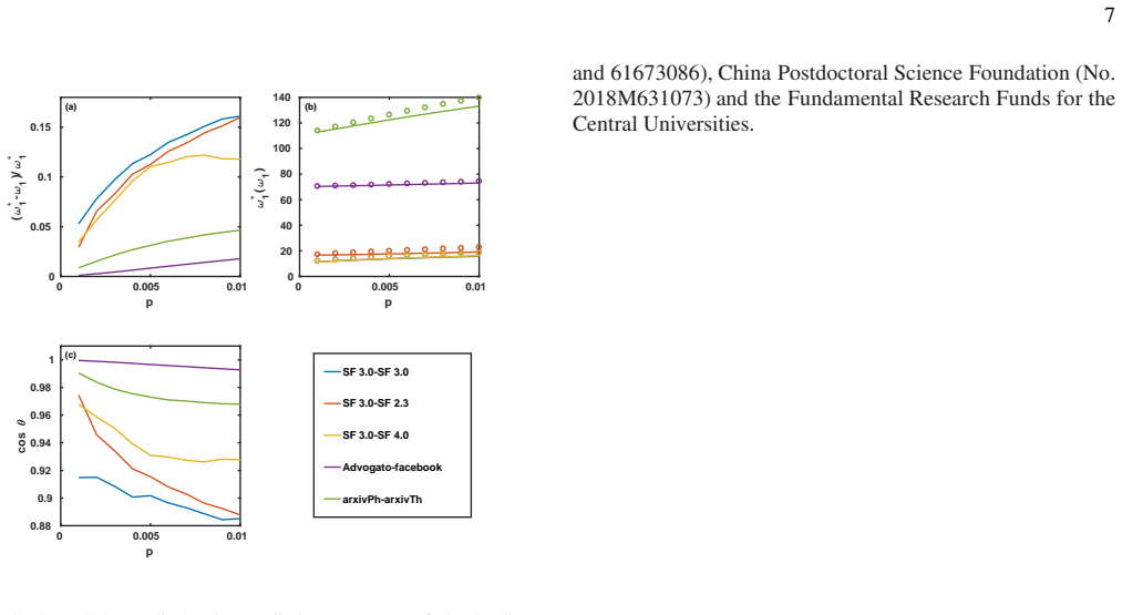
What carries the argument
The LEC strategy, whose load-bearing object is the scalar $E(C) = \langle v_1^a, C v_1^b \rangle$, the sum of products of eigenvector centralities across the chosen inter-layer edges. With the approximation $u \approx u_0$, the leading eigenvalue shift is $\delta\omega_1 = \tfrac{1}{2}(\sqrt{4E(C)^2 + g^2} - g)$, where $g = \omega_1^a - \omega_1^b$, and the prevalence depends on $C$ only through $E(C)$. This turns a combinatorial search over candidate edge sets into a simple ranking problem; the paper then checks monotonicity in $E(C)$ and selects the top-ranked edges.
What would settle it
On a network pair with comparable leading eigenvalues and high modularity, add LEC edges and compare the true leading eigenvector with $u_0$; if the cosine similarity drops well below 1 or the predicted prevalence ordering reverses relative to LDC, the spectral approximation and with it the rule is falsified in that regime.
Extended reading notes
Core claim
For two layers with adjacency matrices $G_a$ and $G_b$ and principal eigenvectors $v_1^a$, $v_1^b$, the paper approximates the leading eigenpair of the interconnected network by taking the leading eigenvector as $u_0 = \beta_a \hat{v}_1^a + \beta_b \hat{v}_1^b$. All dependence of the stationary prevalence on the inter-layer connection matrix $C$ then enters through the single scalar $E(C) = \langle v_1^a, C v_1^b \rangle$. Since the near-critical prevalence and the threshold shift $\delta\omega_1$ are increasing in $E(C)$ for the cases considered, the optimal strategy is to choose the $\delta M$ edges with the largest values $v_1^a(i) v_1^b(j)$. The paper calls this LEC and verifies that it outperforms large-degree and random connecting near the critical point.
Load-bearing premise
The derivation assumes the interconnected network's leading eigenvector is well approximated by the fixed linear combination $\beta_a \hat{v}_1^a + \beta_b \hat{v}_1^b$, with the correction $\delta u$ negligible; if that fails, the reduction of the optimization to $E(C)$ and the LEC rule does not follow.
Editorial extensions
If this is right
- Near the epidemic threshold, LEC outperforms large-degree and random connection strategies for small added-edge budgets across all five tested network pairs.
- The LEC structure that maximizes prevalence also minimizes the outbreak threshold, so a single design rule serves both promotion and containment objectives.
- On synthetic scale-free networks LEC and LDC nearly tie, but on the real-world pairs with complex structure LEC has a clear advantage near threshold.
- Away from the critical point and for very large added-edge counts, the linear approximation degrades and LDC or RC can take over.
Reading between the lines
- Because $E(C)$ is bilinear in the two layer eigenvectors, the top-product rule is a rank-1 approximation to a constrained quadratic assignment; on small instances one could test whether exact enumeration ever beats LEC, and if so how large the gap is.
- The same spectral reduction may carry over to other dynamics controlled by the leading eigenpair, such as synchronization or network reliability, replacing prevalence with the relevant spectral objective.
- A refined strategy for high-modularity, low-average-degree layers could keep the $\delta u$ correction term instead of dropping it; that would yield a testable prediction for when LEC should fail.
Signed reviews
Editorial analysis
A structured set of objections, weighed in public.
Referee Report
Summary. The paper studies how to add a fixed small number of inter-layer edges between two isolated networks so as to maximize the stationary prevalence of the susceptible-infected-susceptible (SIS) model near the epidemic threshold. Using the quenched mean-field formula of Eq. (8), the authors approximate the leading eigenvalue and eigenvector of the interconnected adjacency matrix by a two-dimensional projection onto the two principal eigenvectors, obtaining an expression in which the prevalence depends on the inter-layer matrix C only through E(C)=<v_a1, C v_b1>. Maximizing E(C) leads to the 'large eigenvector connecting' (LEC) rule: connect pairs with the largest products of eigenvector centralities. The rule is tested against large-degree connecting (LDC) and random connecting (RC) on three synthetic and two real-world network pairs, with LEC reported to give the largest prevalence increase near the critical point. The paper concludes that LEC is the optimal inter-layer structure and that it simultaneously minimizes the outbreak threshold.
Significance. If the optimality claim were established, the paper would provide a simple and useful criterion for designing interconnected networks to promote spreading, extending earlier single-edge results to multiple edges. The derivation in Sec. III is transparent, and the numerical comparison in Figs. 3 and 4 is clearly presented and consistent with LEC being a good heuristic near criticality for the tested networks. However, the central claim is stronger than what is demonstrated: the approximation neglects a potentially non-negligible eigenvector correction, the monotonicity of prevalence in E(C) is asserted empirically rather than proven, and optimality is tested only against two heuristics rather than over the full space of edge sets. These gaps do not appear fatal to the heuristic value of LEC, but they do mean that the paper currently establishes 'better than LDC and RC near criticality within a two-eigenvector approximation', not unconditional optimality.
major comments (4)
- [Sec. III, Eqs. (12)-(17)] The reduction of the prevalence to a function of E(C) rests on neglecting the eigenvector correction δu. The justification given in the text is that the leading eigenvalue of scale-free networks diverges in the thermodynamic limit, so that δu is small. This is an asymptotic statement and is not verified for the finite networks used here, particularly Facebook, which has mean degree 2.06 and modularity 0.809 and is far from the divergent-eigenvalue regime. Please provide a quantitative estimate of ||δu||/||u0|| and of the neglected terms in Eq. (18) for all five network pairs as a function of p, and state explicitly the range of p and λ over which Eq. (25) is accurate. Without such a check, the central reduction of the optimization problem to E(C) is not established for the real-world cases.
- [Sec. III, after Eq. (26)] The step from '⟨ρ⟩ depends on C only through E(C)' to 'therefore maximize E(C)' uses the assertion that ⟨ρ⟩ is an increasing function of E(C), which is described as empirical ('Empirically, for all the networks considered...'). This monotonicity is load-bearing: if it fails, a smaller E(C) could give a larger prevalence and the LEC rule would not follow. Please show the actual curve of ⟨ρ⟩ versus E(C) over the candidate range for each network pair, either from Eq. (26) or from iterating Eq. (4), and either prove the monotonicity or specify the exact interval of E(C) where it holds. The Discussion already concedes non-monotonicity for large E(C), so the domain restriction must be quantified.
- [Secs. III-IV, Figs. 3-4] The word 'optimal' is used in the abstract, Sec. I, and Sec. V, but the numerical evidence compares LEC with only two heuristics, LDC and RC. The cosine-similarity check in Fig. 2 is performed on LEC-chosen edge sets, so it does not test whether a different edge set would yield a larger prevalence. Please provide an exhaustive comparison for at least small δM on small synthetic instances (for example, δM = 1 and 2, or a greedy marginal-gain search) or, alternatively, revise the title, abstract, and discussion to claim only 'near-optimal within the stated approximation and better than LDC/RC near criticality'.
- [Sec. III, Eqs. (13)-(14)] The power-method limit u = lim_{n→∞}(ω_a1)^{-n} G^n u0 is approximated by a single application of G (n=1). This is a separate approximation whose error is not bounded. The contributions of δG acting on non-principal eigenvectors are discarded along with δu, and their size depends on the spectral gap of G0, which is not characterized for the real networks. Please either bound this term analytically in terms of ||δG|| and the spectral gap or test its magnitude numerically on the finite networks used in the paper.
minor comments (5)
- [Sec. IV, Fig. 1] In the text and caption, 'expect Advogato-Facebook' should be 'except Advogato-Facebook'.
- [Sec. IV, Eq. (28)] The variability measure is written as the square root of ⟨ρ⟩^2 divided by ⟨ρ⟩^2 minus one; the notation is ambiguous. Please define ⟨ρ⟩^2 explicitly as the mean over independent runs of the squared prevalence and clarify the denominator.
- [Fig. 4 caption] The caption says 'The while lines correspond to the contour'; this should be 'white lines'.
- [Sec. IV, Fig. 3] No error bars are reported for δ⟨ρ⟩. Since the differences between LEC and LDC are small in some panels, please add standard errors or state explicitly that the reported differences are above Monte Carlo noise.
- [Sec. I] The introduction says previous studies mostly considered adding a single edge, but Ref. [42] is later described as generalizing the optimal strategy to two edges. Please clarify precisely which cases are new in the present paper.
Circularity Check
No significant circularity: the LEC strategy is derived from an approximate eigenvalue calculation and independently checked by Monte Carlo simulation, not assumed or fitted.
full rationale
The paper's derivation chain is self-contained apart from external, non-self-cited inputs. It starts from the discrete-time Markov chain equations (Eq. 4, Ref. [46]) and the known near-critical prevalence formula (Eq. 8, Ref. [45]); these are independent benchmarks, not outputs of the paper. The main theoretical step is the in-paper approximation of the leading eigenvector of the interconnected network as u ≈ u0 = βa v̂a1 + βb v̂b1 and the subsequent reduction of the prevalence to a function of E(C) = ⟨va1, C vb1⟩. The decision to drop δu is justified by the external result that the leading eigenvalue diverges for scale-free networks (Ref. [47]), and no parameter is fitted from simulation data and then renamed as a prediction. The LEC rule is obtained by maximizing the approximate ⟨ρ⟩ over C, and the paper then checks the resulting rule against independent Monte Carlo simulations and against the heuristics LDC and RC. Author self-citations appear mainly as background references (e.g., Refs. [23], [27–30], [36–38], [53–57]) and do not carry the central claim. The known limitations—that the two-eigenvector ansatz is asymptotic and may be less accurate for finite real networks, and that the simulations compare LEC only with LDC and RC—are correctness and scope concerns, not circularity. Therefore no step reduces by construction to its own input.
Assumptions & free parameters
assumptions (4)
- domain assumption The quenched mean-field discrete-time Markov chain equations (Eqs. 4-5) accurately describe the SIS dynamics on the networks considered.
- domain assumption The near-critical prevalence formula ⟨ρ⟩ ≈ (λ* ω1 - 1) Σui / (N Σui^3) (Eq. 8) from Ref. [45] holds.
- ad hoc to paper Adding a small number of inter-layer edges only slightly perturbs the spectrum of G0, and the leading eigenvector of G is a linear combination of va1 and vb1 with correction δu neglected.
- domain assumption The stationarity of the Markov chain (ρi = lim t→∞ ρi(t)) is reached in simulations.
Cite this review
Pith. "Pith review of Optimizing spreading dynamics in interconnected networks." pith.science (2026). https://pith.science/paper/HUBISK2M
@misc{pith2026190803406,
  author       = {Pith},
  title        = {Pith review of: Optimizing spreading dynamics in interconnected networks},
  year         = {2026},
  howpublished = {\url{https://pith.science/paper/HUBISK2M}},
  note         = {Machine review of arXiv:1908.03406}
}
read the original abstract
Adding edges between layers of interconnected networks is an important way to optimize the spreading dynamics. While previous studies mostly focus on the case of adding a single edge, the theoretical optimal strategy for adding multiple edges still need to be studied. In this study, based on the susceptible-infected-susceptible (SIS) model, we investigate the problem of maximizing the stationary spreading prevalence in interconnected networks. For two isolated networks, we maximize the spreading prevalence near the critical point by choosing multiple interconnecting edges. We present a theoretical analysis based on the discrete-time Markov chain approach to derive the approximate optimal strategy. The optimal inter-layer structure predicted by the strategy maximizes the spreading prevalence, meanwhile minimizes the spreading outbreak threshold for the interconnected network simultaneously. Numerical simulations on synthetic and real-world networks show that near the critical point, the proposed strategy gives better performance than connecting large degree nodes and randomly connecting.
Figures


Figures from the paper (1 more)

Reference graph
Works this paper leans on
-
[1]
The corresponding eigenvector for an eigenvalue ωa k is ˆva k = (va k, 0)T , (10) which is by combining va 1 and all-zero vector of length Nb. Similarly, for eigenvalue ωb l , the corresponding eigenvector of G0 is ˆvb l = ( 0, vb l ) T (11) with zero vector of length Na. Now we consider adding a small number of interconnecting edges. By assuming these ed...
-
[2]
Thus δu can be ignored for large enough networks and u is approximated as u ≈ u0
(17) For scale-free networks which we mainly consider in the paper, it has been shown that the leading eigenvalue diverge s in the thermodynamic limit [47]. Thus δu can be ignored for large enough networks and u is approximated as u ≈ u0. Denote the gap by g = ωa 1 − ωb
-
[3]
The leading eigenvalue ω1 of G can be written as ω1 = ωa 1 + δω1, which is ωa 1 plus a correction term δω1. With these approximations we arrive at the following eigenvalue equation ( G0 + δG ) u0 = (ωa 1 + δω1) u0. (18) By definition G0u0 = βaωa 1 ˆva 1 + βbωb 1ˆvb 1, (19) and after some algebra Eq. (
-
[4]
until reaching a tolerated error. We perform Monte-Carlo simulations on the networks generated to compare with the theoretical predictions. Fig. 1 shows how ⟨ρ⟩ changes as a function of λ. The recovery rate is fixed to µ = 0 .5 and as well in the rest of the paper. The density of interconnecting edges is p = 0 .01. In the insets of Fig. 1, the theoretical ...
-
[5]
M. Cai, W. Wang, Y . Cui, and H. E. Stanley, Physica A 490, 1 (2018)
work page 2018
-
[6]
A. Sol´ e-Ribalta, S. G´ omez, and A. Arenas, Physical Review Letters 116, 108701 (2016)
work page 2016
-
[7]
are less accurate. Since mean-field theory ignores dynamical correlations [55], i.e ., ignores dependencies among the states of each node and its neighbors, it has been shown that mean-field theory could be less accurate for real-world networks with high clusteri ng coefficient [56], high modularity [57] and low average degree [58]. As shown in TABLE I, the ...
-
[8]
are less accurate for Advogato-Facebook. In general, quenched mean-field theory still predicts well the simulations, therefore can provide a necessary guarantee for the accuracy of the theory develope d in Sec. III. Next we test the accuracy of predictions for the leading eigenvalue ω1 and eigenvector u of the interconnected network. We consecutively add i...
Show all 69 references
-
[9]
Cozzo, R
E. Cozzo, R. A. Banos, S. Meloni, and Y . Moreno, Physical Review E 88, 050801 (2013)
2013
-
[10]
The first row in Fig. 4, i.e. Fig. 4(a1)-(e1), corresponds to LEC minus LDC for the five network pairs, and the second row (Figs. 4(a2)- (e2)) correspond to LEC minus RC. The contours of ǫ = 1e−6 are shown in the plots to indicate the region when LEC performs better. Here ǫ is n...
-
[11]
Boccaletti, G
S. Boccaletti, G. Bianconi, R. Criado, C. I. Del Genio, J. G´ omez-Garde˜ nes, M. Romance, I. Sendi˜ na-Nadal, Z. Wang, and M. Zanin, Physics Reports 544, 1 (2014)
2014
-
[12]
J. Gao, S. V . Buldyrev, H. E. Stanley, and S. Havlin, Nature Physics 8, 40 (2012)
2012
-
[13]
Kivel¨ a, A
M. Kivel¨ a, A. Arenas, M. Barthelemy, J. P . Gleeson, Y . Moreno, and M. A. Porter, Journal of Complex Networks 2, 203 (2014)
2014
-
[14]
De Domenico, C
M. De Domenico, C. Granell, M. A. Porter, and A. Arenas, Nature Physics 12, 901 (2016)
2016
-
[15]
Di Muro, C
M. Di Muro, C. La Rocca, H. Stanley, S. Havlin, and L. Braunstein, Scientific Reports 6, 22834 (2016)
2016
-
[16]
Di Muro, S
M. Di Muro, S. Buldyrev, H. Stanley, and L. Braunstein, Physical Review E 94, 042304 (2016)
2016
-
[17]
Buono and L
C. Buono and L. A. Braunstein, Europhysics Letters 109, 26001 (2015)
2015
-
[18]
Multiplying ˆva 1 and ˆvb 1 from the left separately gives the following equations βb ⟨ va 1 , Cv b 1 ⟩ = δω1βa, βa ⟨ va 1 , Cv b 1 ⟩ − gβ b = δω1βb
becomes (δG − δω1I) u0 = βbgˆvb 1, (20) where I is the N by N identity matrix. Multiplying ˆva 1 and ˆvb 1 from the left separately gives the following equations βb ⟨ va 1 , Cv b 1 ⟩ = δω1βa, βa ⟨ va 1 , Cv b 1 ⟩ − gβ b = δω1βb. (21) 4 The equations can be written in the form ...
-
[19]
S. V . Buldyrev, R. Parshani, G. Paul, H. E. Stanley, and S. Havlin, Nature 464, 1025 (2010)
2010
-
[20]
J. Y . Kim and K.-I. Goh, Physical Review Letters 111, 058702 (2013)
2013
-
[21]
K.-M. Lee, J. Y . Kim, W.-k. Cho, K.-I. Goh, and I. Kim, New Journal of Physics 14, 033027 (2012)
2012
-
[22]
Z. Wang, L. Wang, A. Szolnoki, and M. Perc, European Physical Journal B 88 (2015), 1504.04359
2015 arXiv
-
[23]
and Eq. ( 24). Clearly when g/E (C) → 0, βa → 1 and the two networks play equal role. Meanwhile if g/E (C) ≫ 0, network a dominates b. Normalizing u to unity and substituting back into (8) gives ⟨ρ⟩ = (λ∗ ωa 1 + λ∗ δω1 − 1) × ( (βa)3 + βa ) θa 1 + ( (βa)2 + 1 ) θb 1 N ( (βa)3 ...
-
[24]
Zhang, S
X. Zhang, S. Boccaletti, S. Guan, and Z. Liu, Physical Review Letters 114, 038701 (2015)
2015
-
[25]
Start with two isolated networks, we consecutively add the edges and do the comparison after each adding
to the true values ω∗ 1 and u∗. Start with two isolated networks, we consecutively add the edges and do the comparison after each adding. To quantify the accuracy, for the leading eigenvalue we consider the relative error (ω∗ 1 − ω1) /ω∗ 1, where ω∗ 1 is the true eigenvalue an...
-
[26]
L. D. V aldez, P . A. Macri, H. E. Stanley, and L. A. Braunstein, Physical Review E 88, 050803 (2013)
2013
-
[27]
V aldez, M
L. V aldez, M. Di Muro, and L. Braunstein, Journal of Statistical Mechanics: Theory and Experiment 2016, 093402 (2016)
2016
-
[28]
Cohen, D
R. Cohen, D. Ben-Avraham, and S. Havlin, Physical Review E 66, 036113 (2002)
2002
-
[29]
M. ´A. Serrano and M. Bogun´ a, Physical Review Letters 97, 088701 (2006)
2006
-
[30]
Goltsev, S
A. Goltsev, S. Dorogovtsev, and J. Mendes, Physical Review E 78, 051105 (2008)
2008
-
[31]
M. Perc, J. J. Jordan, D. G. Rand, Z. Wang, S. Boccaletti, and A. Szolnoki, Physics Reports 687, 1 (2017)
2017
-
[32]
Z. Wang, A. Szolnoki, and M. Perc, Scientific Reports 3 8 0 0.1 0.20 0.005 0.01 0.015δ〈ρ〉 0 0.1 0.20 0.005 0.01 0 0.1 0.20 0.005 0.01 λ 0 0.01 0.020 2 4 6 x 10 −3 λ δ〈ρ〉 0 0.01 0.020 2 4 6 x 10 −3 λ LEC LDC RC µ/ω a 1 (a) (b) (c) (e)(d) FIG. 3. (Color online) δ⟨ρ⟩ versus λ for ...
2013
- [33]
-
[34]
C. D. Brummitt, K.-M. Lee, and K.-I. Goh, Physical Review E 85, 045102 (2012)
2012
-
[35]
K.-M. Lee, C. D. Brummitt, and K.-I. Goh, Physical Review E 90, 062816 (2014)
2014
-
[36]
Ya˘ gan and V
O. Ya˘ gan and V . Gligor, Phys. Rev. E86, 036103 (2012)
2012
-
[37]
Wang, X.-L
W. Wang, X.-L. Chen, and L.-F. Zhong, Physica A 503, 604 (2018)
2018
-
[38]
W. Wang, M. Tang, H. E. Stanley, and L. A. Braunstein, Physical Review E 98, 062320 (2018)
2018
-
[39]
Shu, Q.-H
P . Shu, Q.-H. Liu, S. Wang, and W. Wang, Chaos 28, 113114 (2018)
2018
-
[40]
X. Chen, W. Wang, S. Cai, H. E. Stanley, and L. A. Braunstein, Journal of Statistical Mechanics: Theory and Experiment 2018, 053501 (2018)
2018
-
[41]
Saumell-Mendiola, M
A. Saumell-Mendiola, M. ´A. Serrano, and M. Bogun´ a, Physical Review E 86, 026106 (2012)
2012
-
[42]
Pastor-Satorras and A
R. Pastor-Satorras and A. V espignani, Physical Review Lett ers 86, 3200 (2001)
2001
-
[43]
H. Wang, Q. Li, G. D’Agostino, S. Havlin, H. E. Stanley, and P . V an Mieghem, Physical Review E88, 022801 (2013)
2013
-
[44]
G. F. de Arruda, E. Cozzo, T. P . Peixoto, F. A. Rodrigues, and Y . Moreno, Physical Review X7, 011014 (2017)
2017
-
[45]
Dickison, S
M. Dickison, S. Havlin, and H. E. Stanley, Physical Review E 85, 066109 (2012)
2012
-
[46]
W. Wang, M. Tang, H. Yang, Y . Do, Y .-C. Lai, and G. Lee, Scientific Reports 4, 5097 (2014)
2014
-
[47]
Wang, Q.-H
W. Wang, Q.-H. Liu, S.-M. Cai, M. Tang, L. A. Braunstein, and H. E. Stanley, Scientific Reports 6, 29259 (2016)
2016
-
[48]
Q.-H. Liu, W. Wang, M. Tang, and H.-F. Zhang, Scientific Reports 6 (2016)
2016
-
[49]
Parshani, C
R. Parshani, C. Rozenblat, D. Ietri, C. Ducruet, and S. Havli n, Europhysics Letters 92, 68002 (2011)
2011
-
[50]
Aguirre, D
J. Aguirre, D. Papo, and J. M. Buld´ u, Nature Physics 9, 230 (2013)
2013
-
[51]
Aguirre, R
J. Aguirre, R. Sevilla-Escoboza, R. Guti´ errez, D. Papo, an d J. Buld´ u, Physical Review Letters112, 248701 (2014)
2014
-
[52]
Y . Li, X. Wu, J.-a. Lu, and J. L¨ u, IEEE Transactions on Circuits and Systems II: Express Briefs 63, 206 (2016)
2016
-
[53]
J. Wei, X. Wu, J.-A. Lu, and X. Wei, Europhysics Letters 120, 20005 (2018)
2018
-
[54]
X. Wei, J. Emenheiser, X. Wu, J.-A. Lu, and R. M. D’Souza, Chaos 28, 013110 (2018)
2018
-
[55]
Goltsev, S
A. Goltsev, S. Dorogovtsev, J. Oliveira, and J. Mendes, Physical Review Letters 109, 128702 (2012)
2012
-
[56]
G´ omez, A
S. G´ omez, A. Arenas, J. Borge-Holthoefer, S. Meloni, and Y . Moreno, Europhysics Letters89, 38009 (2010)
2010
-
[57]
K. I. Goh, B. Kahng, and D. Kim, Physical Review E 64, 051903 (2001)
2001
-
[58]
Massa, M
P . Massa, M. Salvetti, and D. Tomasoni, in Dependable, Autonomic and Secure Computing, 2009. DASC’09. Eighth IEEE International Conference on (IEEE, 2009) pp. 658–663
2009
-
[59]
Leskovec and J
J. Leskovec and J. J. Mcauley, in Advances in neural information processing systems (2012) pp. 539–547
2012
-
[60]
Leskovec, J
J. Leskovec, J. Kleinberg, and C. Faloutsos, ACM Transactio ns on Knowledge Discovery from Data (TKDD) 1, 2 (2007). 9 FIG. 4. (Color online) The difference of ⟨ρ⟩ for LEC−LDC in the first row ((a1)-(e1)) and LEC −RC in second row ((a2)-(e2)). Each one of the five columns corresp...
2007
-
[61]
http://konect.uni-koblenz.de/networks/
-
[62]
M. E. Newman, Proceedings of the National Academy of Sciences 103, 8577 (2006)
2006
-
[63]
P . Shu, W. Wang, M. Tang, and Y . Do, Chaos 25, 063104 (2015)
2015
-
[64]
P . Shu, W. Wang, M. Tang, and P . Zhao, Chaos 26, 063108 (2016)
2016
-
[65]
W. Wang, M. Tang, H. E. Stanley, and L. A. Braunstein, Reports on Progress in Physics 80, 036603 (2017)
2017
-
[66]
Radicchi and C
F. Radicchi and C. Castellano, Physical Review E 93, 030302 (2016)
2016
-
[67]
Wang, Q.-H
W. Wang, Q.-H. Liu, L.-F. Zhong, M. Tang, H. Gao, and H. E. Stanley, Scientific Reports 6, 24676 (2016)
2016
-
[68]
J. P . Gleeson, S. Melnik, J. A. Ward, M. A. Porter, and P . J. Mucha, Physical Review E 85, 026106 (2012)
2012
-
[69]
L. L¨ u, D. Chen, X.-L. Ren, Q.-M. Zhang, Y .-C. Zhang, and T. Zhou, Physics Reports 650, 1 (2016)
2016
Reviewed August 14, 2026 · model on record in the stance chip above.
Discussion (0). Continue with ORCID to comment.