Spatial Flow-Field Approximation Using Few Thermodynamic Measurements Part I: Formulation and Area Averaging

Andrew Duncan; Duncan Simpson; Geoffrey Parks; George Thorne; Pranay Seshadri

REVIEW 3 major objections 5 minor 18 references

Spatial Flow-Field Approximation Using Few Thermodynamic Measurements Part I: Formulation and Area Averaging

T0 review · 3 major / 5 minor · reviewed 2026-08-14 · deepseek-v4-flash

Challenge this review Re-run · record.json Download PDF Read on arXiv ↗ Review JSON

Pith's one-line read A two-harmonic temperature model can recover true area averages from sparse engine measurements.

desk verdict Useful engineering recipe with a genuine held-out test, but the controlled validation contains an arithmetic contradiction that blocks the central claim as written. read the letter →

arxiv 1908.03431 v1 pith:WUJNCFHX submitted 2019-08-08 stat.AP

Pranay Seshadri , Duncan Simpson , George Thorne , Andrew Duncan , Geoffrey Parks This is my paper · ORCID

classification stat.AP

keywords enginetemperaturemeasurementsspatialfieldreconstructionareaaveragingFourierharmonicsTikhonovregularizationcross-validationsparsethermocoupledataturbomachinery

verification ladder T0 review T1 audit T2 compute T3 formal

The pith

A machine-rendered reading of the paper's core claim, the machinery that carries it, and where it could break.

The reading

The paper claims that from a handful of thermocouple rakes at one axial plane, a regularized linear model with just two circumferential Fourier harmonics and a quadratic radial polynomial can reconstruct the two-dimensional temperature field well enough to compute a trustworthy area average. The claim is tested on 82 data-sets from five similar engines, with held-out rake cross-validation on the eight-rake engine showing that the harmonic pair $\omega=(1,4)$ gives the lowest prediction error. The central point is that the model need not capture every spatial harmonic: because the area average integrates out all nonzero circumferential modes, a low-order fit can still deliver the true average if its constant circumferential term is right. If correct, this gives a practical, parameter-light route from sparse engine test data to spatial temperature maps and area averages.

What carries the argument

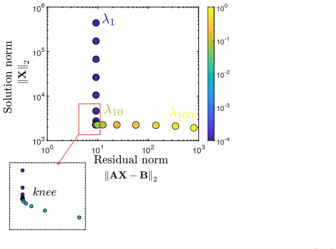
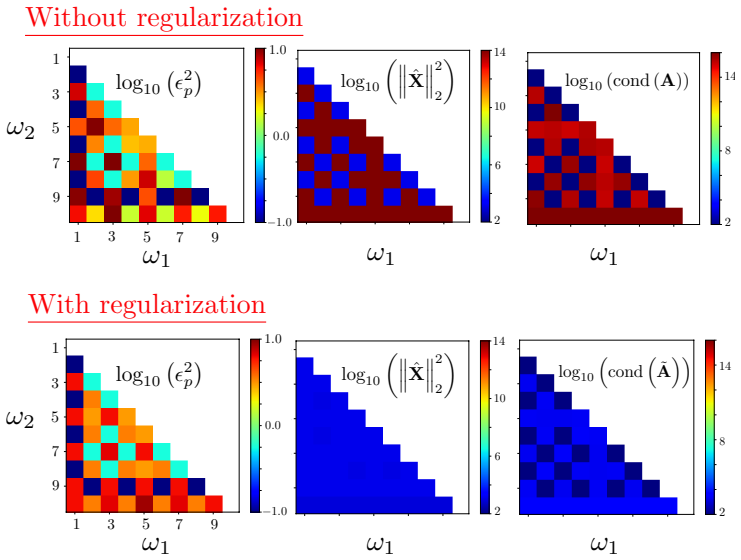
The carrying object is the parametric field model $T(r,\$\theta$)=v^T(r)UX^Ta(\$\theta$)$, where $a(\$\theta$)$ contains the Fourier basis for the chosen circumferential harmonics, $X$ holds the harmonic coefficients at each measured radial tap, and $v(r)$ is the quadratic radial polynomial basis. Tikhonov regularization with the L-curve criterion keeps the fitted coefficients small and prevents unphysical oscillation between rakes. The mechanism that makes the averaging claim work is that the circumferential integral in the area-average formula kills every nonzero Fourier harmonic, so the area average depends only on the mean, constant term of the fitted field; if the low-order fit recovers that constant term, the average is correct even when individual harmonics are aliased or wrong.

What would settle it

Take a real or simulated temperature field with significant energy at circumferential frequencies above 10 and sharp radial gradients, sample it at the rake positions in Table 1, fit the two-harmonic quadratic model, and compare the model area average with a high-resolution numerical area average of the true field; a discrepancy well above 2 K would refute the claim that low-order fits can still deliver the true average.

Watch

Extended reading notes

Core claim

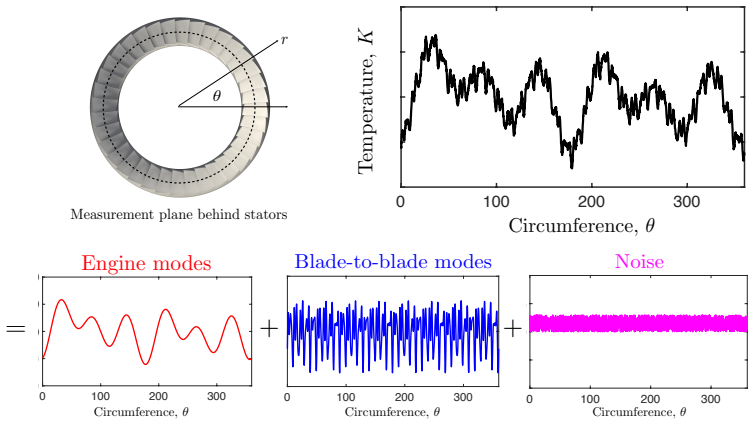
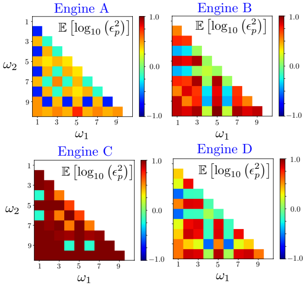
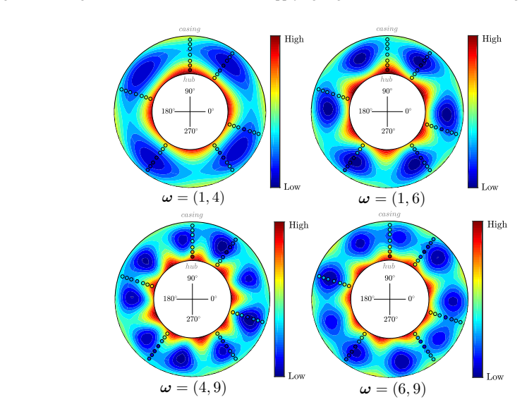
The authors' central claim is that a regularized linear model with two circumferential Fourier harmonics and a quadratic radial polynomial, fitted to a few thermocouple rakes at one axial plane, can reconstruct the two-dimensional temperature field well enough to compute a meaningful area average. Across 82 extracts from five engines of the same family, the harmonic pair $\omega=(1,4)$ consistently gives the lowest held-out prediction error when two of eight rakes on Engine E are reserved for testing. On an analytically generated profile containing four harmonics, the same pair recovers the dominant spatial pattern without capturing the higher harmonics, and its area average matches the true profile average. On the engine data, area averages computed from the fitted fields differ from sector-weighted averages by 0.5 to 2 K. The authors conclude that the model need not capture every spatial harmonic; in some cases it can still deliver the true area average.

Load-bearing premise

The method assumes the true temperature field is dominated by two low-frequency circumferential patterns, with frequency at most 10, and a smooth radial variation; if a real engine has substantial faster or sharper variation, those patterns will be folded into the fitted low-order coefficients and the field and its average will be wrong.

Editorial extensions

If this is right

The paired frequency-selection and regularization approach gives engine-test engineers a parameter-light way to produce full 2D temperature maps from the six or eight rakes already installed.
Area averages from the fitted field can serve as an alternative to sector-weighted averaging, with a quantified agreement of 0.5 to 2 K on five similar engines.
Because the model intentionally fits only low circumferential harmonics, the resulting maps isolate engine modes from blade-to-blade modes, which is exactly the information rigs and CFD cannot supply.
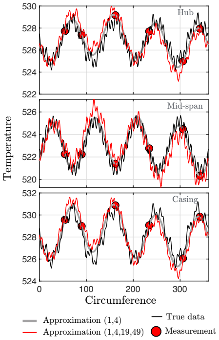
The assumed-profile study shows that even when higher harmonics are present, a six-rake fit with $\omega=(1,4)$ plus a minimum-norm correction can approximate the true circumferential temperature profile at representative span positions.

Reading between the lines

Editorial extensions of the paper, not claims the author makes directly.

If the constant-term mechanism holds generally, the same approach should transfer to any circumferentially averaged quantity, such as pressure or species concentration, whenever the averaging operator annihilates the omitted harmonics; a direct test would be to build synthetic fields with energy above $\omega=10$ and check how large the average error becomes.
The 0.5 to 2 K spread likely tracks how well the quadratic radial basis captures the true radial profile and how favorably the rakes sample the constant term; adding a third radial degree or optimizing rake placement could shrink the spread, but the paper does not test this.
The frequency-selection recipe could be inverted into a sensor-placement rule: choose rake positions that make the Fourier matrix well-conditioned for $\omega=(1,4)$, since that pair already wins held-out tests; the paper does not pursue this optimization.

Share X Bluesky LinkedIn Reddit HN

Signed reviews

No signed human review yet.

Editorial analysis

A structured set of objections, weighed in public.

Desk editor's note, referee report, and a circularity audit.

Desk Editor's Note

read the letter

The paper is worth your time if you work with sparse turbomachinery thermocouple data. It assembles standard tools—ridge regression, Fourier basis, radial polynomial, L-curve selection—into a 2D reconstruction-and-averaging workflow, and it validates the harmonic choice with held-out rakes on a fifth engine. That held-out test is the strongest part: across 28 rake splits, (1,4) does minimize prediction error, and the framework gives a concrete way to turn a few rakes into a spatial field and a sector-aware average.

The soft spots are real but mostly addressable. The most serious is the controlled case study in Sec. 4. The assumed profile's true average is stated as 526.85 K, the sector-weighted average as 526.20 K, and the fitted (1,4) model as 525.85 K. The text then says the model average is "greater than the area weighted value" and "equivalent to the profile average temperature value." Both statements are arithmetically false: 525.85 is less than both 526.20 and 526.85. Since this is the only place where the "true area average" claim is checked against ground truth, the central claim is not demonstrated as written. This could be a typo or round-off issue, but it is load-bearing and must be corrected and re-verified before the claim can stand.

Two other issues are worth noting. First, the four candidate harmonic pairs were preselected from Engines A-D and then pruned on Engine E; the test on E is legitimate, but the selection step is not accounted for, so the reported errors are somewhat optimistic. Nested cross-validation would fix this. Second, the model class restricts max frequency to 10 and the radial polynomial to quadratic. If a real engine has significant energy at higher circumferential or radial modes, those modes can alias into the fitted coefficients, including the constant term that determines the area average; leave-rake-out CV cannot detect this because the candidate set never includes those frequencies. The paper's own discussion of aliasing does not address this particular risk.

The math is standard but used correctly, the citation pattern is fine, and the paper is honest about its two-part structure. The methodology itself is not fatally flawed; the Sec. 4.3 discrepancy is an arithmetic error, not an incoherent argument. I would send this to peer review, but with the discrepancy flagged as a mandatory revision, and with a request for uncertainty quantification on the reported averages and a clear statement about the model-class limitation. For now, I would not cite the 0.5–2 K claim until the contradiction is resolved. Read it for the formulation and the cross-validation design; treat the quantitative claims with caution.

Referee Report

3 major / 5 minor

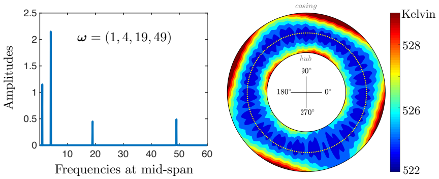
Summary. The paper develops a regularized multivariate linear regression model for reconstructing the 2D temperature field at a fixed axial plane in a turbofan engine from a small number of circumferentially placed thermocouple rakes. The model uses a Fourier basis in the circumferential direction and a quadratic polynomial in the radial direction, with Tikhonov regularization and a brute-force search over two-harmonic frequency pairs. Using 70 extracts from Engines A–D, the authors identify four candidate frequency pairs, and a leave-two-rakes-out cross-validation on Engine E is used to argue that the pair ω=(1,4) has the lowest predictive error. An assumed analytical temperature profile with harmonics (1,4,19,49) is used to test whether a two-harmonic model can recover the true area average; the paper reports an area average of 525.85 K from the fitted model and claims it is equivalent to the true profile average of 526.85 K. The central conclusion is that the fitted model need not capture all spatial harmonics but can still deliver the true area average.

Significance. If the central claim were established, the paper would provide a practical and computationally cheap method for reconstructing sparse engine temperature fields and computing area averages from them, which is relevant to turbomachinery instrumentation practice. The paper has genuine strengths: the formulation in Sec. 3 is explicit and reproducible in structure; Eq. (21) gives a clean analytical expression showing that the area average depends only on the constant Fourier coefficient after radial integration; and the leave-rakes-out experiment on Engine E is a sensible holdout device. However, the headline claim is not currently supported as written. The single controlled validation contains an internal numerical contradiction, and the model-class restriction to two harmonics with max frequency ≤10 means that aliasing of unmodeled modes could bias the very constant term that determines the area average. The significance is therefore conditional: the method is promising, but the evidence for its unbiased averaging property needs correction and strengthening.

major comments (3)

[Sec. 4, Sec. 4.3, Conclusions] The controlled validation of the central area-averaging claim contains an internal arithmetic contradiction. The assumed profile is stated to have an average temperature of 526.85 K (Sec. 4), the sector-weighted average is reported as 526.20 K, and the fitted (1,4) model area average is reported as 525.85 K (Sec. 4.3). The text then says that 525.85 K is 'greater than the area weighted value' and 'equivalent to the profile average temperature value.' Both statements are false as written: 525.85 < 526.20 < 526.85. Since this controlled example is the only place where the fitted model's area average is compared to a known true average, the paper does not demonstrate the conclusion that a two-harmonic model 'can still deliver the true area average.' The numbers must be corrected, or, if the 1 K difference is considered acceptable, the paper must state an explicit tolerance and justify it in the context of engine temperature measurement uncertainty.
[Sec. 3.3, Sec. 4, Eq. (21)] The model-class restriction is load-bearing for the averaging claim but is not tested against it. The search is restricted to two harmonics with max{ω}≤10, and the radial dependence is a quadratic polynomial. Because Eq. (21) shows that the area average depends only on the estimated constant Fourier coefficient, any aliasing of true higher harmonics (e.g., ω=19 and 49 in the assumed profile) into that constant term directly biases the area average. The paper's only controlled case does show a 1 K discrepancy between 525.85 K and the true 526.85 K, which is consistent with such bias; the Engine E cross-validation cannot detect this because the candidate set never contains the higher frequencies. To support the conclusion, the authors should either prove a condition under which the fitted constant term is unbiased despite aliasing, or demonstrate numerically on an ensemble of profiles with varied higher-harmonic content that the area-average error remains within a stated tolerance.
[Sec. 3.5, Fig. 7] The cross-validation on Engine E is partly a model-selection step, not an independent test of the final selected model. The four candidate frequency pairs were pre-selected from Engines A–D, and then Engine E is used to 'further prune down' the harmonics; the claim that ω=(1,4) minimizes ε_test is the output of that pruning. Consequently the reported test errors are not unbiased estimates of the generalization error of the final model, and the comparison in Fig. 7 does not by itself establish that (1,4) is the best pair for unseen data. The authors should either use a nested procedure (select on A–D, evaluate once on E) or explicitly frame Fig. 7 as descriptive model comparison and temper the claim accordingly.

minor comments (5)

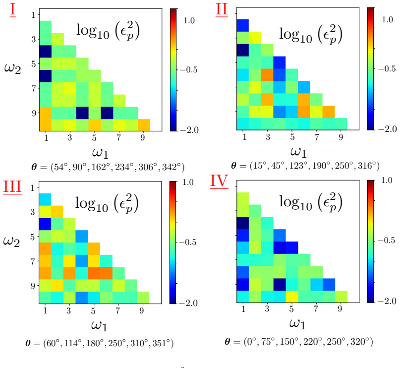
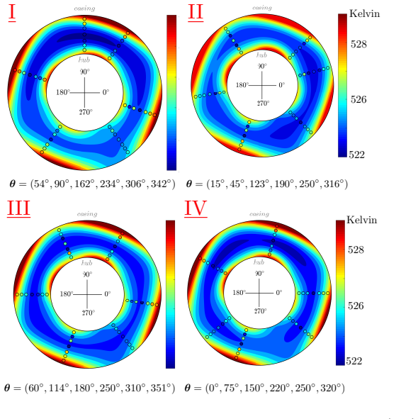
[Sec. 4, Table 2] Table 2, Case I is described as being based on the Engine A arrangement, but the listed rake positions (54°, 90°, 162°, 234°, 306°, 342°) match Engines B, C, and D in Table 1, not Engine A, which has 270° in place of 306°. Please correct either the table entry or the description.
[Sec. 4.3, Eq. (21)] Equation (21) contains a typographical double equals sign ('Tavge = = 1/(π(...))'); this should be cleaned up.
[Sec. 3.2] The radial polynomial degree p is not explicitly specified; the text refers to a 'quadratic polynomial' but Eq. (6) leaves p general. Please state p=3 explicitly and define M, the number of radial probes per rake, in the notation of Sec. 3.2.
[Sec. 3.3] In Algorithm 1, the relationship between the constraint β in problem (12) and the fixed set of λ values (0.0001, 0.001, 0.1, 10) is not stated; the while loop appears to select among these four values, but the stopping criterion and the choice of β are not tied to the optimization formulation. A brief clarification would improve reproducibility.
[References] Reference [9] contains a typographical artifact in the author list ('Seshadri, P., , Duncan, A.'); the missing author initial or comma should be fixed.

Circularity Check

0 steps flagged · score 0.0 of 10

No significant circularity: the regression, harmonic selection, and area-average derivations are self-contained, though the assumed-case demonstration contains a numerical inconsistency that is a correctness issue rather than a circular one.

full rationale

The paper's derivation chain is mostly self-contained. The model coefficients X are fitted from measurement matrix B via Eqs. (3)/(14); the radial polynomial is fitted via Eq. (7). Harmonic pairs are first screened on Engines A-D (Fig. 4), then compared on Engine E using leave-P-out cross-validation where the held-out rakes are not used to fit X (Eqs. 16-18). This is a genuine out-of-sample comparison, not a fitted parameter renamed as a prediction. The assumed case study in Sec. 4 is an externally defined analytic profile with an independently stated average temperature of 526.85 K and harmonics (1,4,19,49), so testing whether (1,4) recovers the dominant modes and whether Eq. (21) gives the correct average is a validation against independent ground truth, not a circular reduction. Eq. (21)'s conclusion that the area average depends only on the constant Fourier term follows from Fourier orthogonality and is a first-principles identity. No load-bearing step is justified by a self-citation chain: reference [9] merely points to a companion paper and is not used to force any conclusion. The only serious flaw is in Sec. 4.3: the text reports the fitted area average as 525.85 K and calls it greater than the sector-weighted 526.20 K and equivalent to the profile average 526.85 K, both of which are arithmetically wrong. This undermines the demonstrated support for the central averaging claim, but it is an evidentiary/correctness problem, not a circularity.

Assumptions & free parameters 6 free parameters · 5 assumptions · 1 invented entities

Everything the central claim rests on beyond the raw thermocouple measurements is listed above. The free-parameter count is high relative to the simplicity of the model: the harmonic search bound, the λ list, the β bound, and the radial degree are all chosen by hand, and the four surviving frequency pairs are selected post hoc from the same engines used to report low errors. The domain assumptions are all reasonable for turbomachinery, but they are stated rather than demonstrated. The one invented entity, the synthetic profile, is the only place an external 'truth' is available, and it is constructed to contain the answer. Net contribution: the paper adds a workflow and an empirical finding; the priors (basis class, spectral separation of modes, engine-family similarity) are pulled from domain knowledge rather than derived.

free parameters (6)

Maximum circumferential frequency bound = 10
Imposed to 'focus on lower harmonics' (Sec. 3.3); no principled justification, and it caps the candidate set, so aliasing from ω>10 is never tested. This directly shapes the empirical finding that (1,4) is best.
Regularization strengths λ = list {0.0001, 0.001, 0.1, 10}; L-curve knee (Fig. 2)
Algorithm 1 steps λ through an ad-hoc four-value list until the norm constraint is met; the L-curve 'knee' is a visual choice. Different λ lists would change which frequency pairs survive the selection.
Solution-norm bound β = 10^5
The constraint ||X||² ≤ β² with β=10^5 is fixed by hand for all 70 training extracts (Sec. 3.4); no sensitivity analysis is given.
Number of harmonics k = 2
Forced by N=6 rakes through the constraint N > 2k+1 (Sec. 3.3), not by a physics or model-selection argument; the model class is therefore the two-frequency class.
Candidate harmonic pairs = (1,4), (1,6), (4,9), (6,9)
Selected post hoc from the average error maps of Engines A-D as 'consistently yield low errors' (Sec. 3.4, Fig. 4) with no multiple-comparison control; these four, rather than all pairs, are what gets tested on Engine E.
Radial polynomial degree = p=3 (quadratic)
The radial model is declared quadratic (Sec. 3.2) without model selection or a stated basis for the degree.

assumptions (5)

domain assumption The temperature field is a superposition of engine modes, blade-to-blade modes, and noise, with engine modes at low frequencies.
Figure 1 and Sec. 1; the harmonic-selection program is only meaningful if this spectral separation holds.
domain assumption Five engines with similar architectures have similar temperature spatial harmonics.
Abstract and Sec. 3.5 (footnote); training harmonics on A-D and applying them to E, and to the family, depends on this transfer.
domain assumption Rake positions avoid stator vane wakes, so the sampled field represents engine modes rather than being dominated by blade-to-blade structure.
Sec. 3.1: rakes are 'circumferentially positioned to avoid the wakes associated with these vanes.'
domain assumption Temporal-averaging measurement uncertainties are negligible.
Sec. 3.1 makes this assumption explicitly; all uncertainty quantification is deferred to the companion paper.
standard math Fourier harmonic terms integrate to zero over 0 to 2π, leaving only the constant term in the area average.
Used in Eq. (21), Sec. 4.3, to reduce the area average to a radial integral of the first column of X^T.

invented entities (1)

Assumed analytical temperature profile with harmonics ω=(1,4,19,49)
purpose: Synthetic validation object used to test harmonic recovery and to support the claim that the model area average equals the true average.
The profile is constructed by the authors (Sec. 4, Fig. 8) with harmonics 1 and 4 dominant, so the finding that the method selects (1,4) for it is a property of the construction, not an external check.

how reviews work

0 comments

Cite this review

Pith. "Pith review of Spatial Flow-Field Approximation Using Few Thermodynamic Measurements Part I: Formulation and Area Averaging." pith.science (2026). https://pith.science/paper/WUJNCFHX

@misc{pith2026190803431,
  author       = {Pith},
  title        = {Pith review of: Spatial Flow-Field Approximation Using Few Thermodynamic Measurements Part I: Formulation and Area Averaging},
  year         = {2026},
  howpublished = {\url{https://pith.science/paper/WUJNCFHX}},
  note         = {Machine review of arXiv:1908.03431}
}

read the original abstract

Our investigation raises an important question that is of relevance to the wider turbomachinery community: how do we estimate the spatial average of a flow quantity given finite (and sparse) measurements? This paper seeks to advance efforts to answer this question rigorously. In this paper, we develop a regularized multivariate linear regression framework for studying engine temperature measurements. As part of this investigation, we study the temperature measurements obtained from the same axial plane across five different engines yielding a total of 82 data-sets. The five different engines have similar architectures and therefore similar temperature spatial harmonics are expected. Our problem is to estimate the spatial field in engine temperature given a few measurements obtained from thermocouples positioned on a set of rakes. Our motivation for doing so is to understand key engine temperature modes that cannot be captured in a rig or in computational simulations, as the cause of these modes may not be replicated in these simpler environments. To this end, we develop a multivariate linear least squares model with Tikhonov regularization to estimate the 2D temperature spatial field. Our model uses a Fourier expansion in the circumferential direction and a quadratic polynomial expansion in the radial direction. One important component of our modeling framework is the selection of model parameters, i.e. the harmonics in the circumferential direction. A training-testing paradigm is proposed and applied to quantify the harmonics.

Figures

Figures reproduced from arXiv: 1908.03431 by the authors.

**Figure 2.** The L-curve for the regularized least squares problem on an extract from Engine A with [PITH_FULL_IMAGE:figures/full_fig_p008_2.png] view at source ↗

**Figure 3.** Brute force frequency selection with and without regularization for the last extract from the Engine A data-set. [PITH_FULL_IMAGE:figures/full_fig_p009_3.png] view at source ↗

Figures from the paper (8 more)

**Figure 4.** Figure 4: Average values of the RMS error when applying Algorithm 1 to the data-sets of Engines A, B, C and D. [PITH_FULL_IMAGE:figures/full_fig_p010_4.png]

**Figure 5.** Figure 5: Spatial representations of the temperature shown for the first extract in Engine A. The contour bounds are set [PITH_FULL_IMAGE:figures/full_fig_p010_5.png]

**Figure 6.** Figure 6: Testing the multivariate regression model on Engine E with certain rakes reserved for training and the re [PITH_FULL_IMAGE:figures/full_fig_p011_6.png]

**Figure 8.** Figure 8: An assumed temperature profile with four harmonics; the amplitude and phases are varied from hub to casing. [PITH_FULL_IMAGE:figures/full_fig_p013_8.png]

**Figure 9.** Figure 9: Values of the error ε 2 for four different sets of rake positions. 14 [PITH_FULL_IMAGE:figures/full_fig_p014_9.png]

**Figure 10.** Figure 10: Temperature profiles for four different rake positions with [PITH_FULL_IMAGE:figures/full_fig_p015_10.png]

**Figure 11.** Figure 11: An assumed temperature profile with four harmonics; the amplitude and phases are varied from hub to [PITH_FULL_IMAGE:figures/full_fig_p016_11.png]

**Figure 12.** Figure 12: Workflow from thermocouple measurements to a spatial average. [PITH_FULL_IMAGE:figures/full_fig_p017_12.png]

Discussion (0). Continue with ORCID to comment.

Reference graph

Works this paper leans on

18 extracted references · 17 canonical work pages

[1]

Analysis of rotor-stator-interaction and blade- to-blade measurements in a two stage axial ﬂow compressor

Ernst, M., Michel, A., and Jeschke, P., 2011. “Analysis of rotor-stator-interaction and blade- to-blade measurements in a two stage axial ﬂow compressor”.Journal of Turbomachinery, 133(1), p. 011027

work page 2011
[2]

Multi-blade row interactions in a transonic axial compressor Part I: Stator particle image velocimetry (PIV) investigation

Sanders, A., Papalia, J., and Fleeter, S., 2002. “Multi-blade row interactions in a transonic axial compressor Part I: Stator particle image velocimetry (PIV) investigation”.Journal of Turbomachinery, 124, pp. 10–18

work page 2002
[3]

Periodical unsteady ﬂow within a rotor blade row of an axial compressor Part I: Flow ﬁeld at midspan

Mailach, R., Lehmann, I., and Vogeler, K., 2008. “Periodical unsteady ﬂow within a rotor blade row of an axial compressor Part I: Flow ﬁeld at midspan”.Journal of Turbomachinery, 130(4), p. 041004

work page 2008
[4]

W., and Arnaiz, H

Stoll, F., Tremback, J. W., and Arnaiz, H. H., 1979. Eﬀect of Number of Probes and their Orientation on the Calculation of Several Compressor Face Distortion Descriptors. Tech. rep., NASA Technical Memorandum 72859

work page 1979
[5]

T., and Morse, I

Francis, S. T., and Morse, I. E., 1989.Measurement and Instrumentation in Engineering: Principles and Basic Laboratory Experiments, Vol. 67. CRC Press, Boca Raton, FL. 18

work page 1989
[6]

Averagingnonuniformﬂowforapurpose

Cumpsty,N.A.,andHorlock,J.H.,2006.“Averagingnonuniformﬂowforapurpose”. Journal of Turbomachinery, 128(1), pp. 120–129

work page 2006
[7]

Suitable Averaging Techniques in Non-Uniform Internal Flows

Pianko, M., and Wazelt, F., 1983. Suitable Averaging Techniques in Non-Uniform Internal Flows. Tech. rep., AGARD-AR-182

1983
[8]

Consistent mean values for compressible media in the theory of turbo- machines

Dzung, L. S., 1971. “Consistent mean values for compressible media in the theory of turbo- machines”.Brown Boveri Review, 58(10), pp. 485–492

work page 1971

Show all 18 references

[9]

Spatial ﬂow-ﬁeld approximation using few thermodynamic measurements Part II: Uncertainty assessments

Seshadri, P., , Duncan, A., Simpson, D., Thorne, G., and Parks, G., 2019. “Spatial ﬂow-ﬁeld approximation using few thermodynamic measurements Part II: Uncertainty assessments”. Submitted to ASME Journal of Turbomachinery

2019
[10]

W., 1980

Skiles, T. W., 1980. Turbine Engine Flowpath Averaging Techniques. Tech. rep., Arnold Air Force Station, Texas

1980
[11]

Reducing instrumentation errors caused by circumferential ﬂow ﬁeld variation in multi-stage axial compressors

Chilla, M., Pullan, G., and Gallimore, S., 2019. “Reducing instrumentation errors caused by circumferential ﬂow ﬁeld variation in multi-stage axial compressors”. In ASME Turbo Expo 2019: Turbomachinery Technical Conference and Exposition, American Society of Mechan- ical Engin...

2019
[12]

The Elements of Statistical Learning,2nded

Hastie,T.,Tibshirani,R.,andFriedman,J.,2009. The Elements of Statistical Learning,2nded. Series in Statistics. Springer, New York, NY

2009
[13]

CRC Press, Boca Raton, FL

Rogers, S., and Girolami, M., 2016.A First Course in Machine Learning . CRC Press, Boca Raton, FL

2016
[14]

MIT Press, Cambridge, MA

Goodfellow, I., Bengio, Y., and Courville, A., 2016.Deep Learning. MIT Press, Cambridge, MA

2016
[15]

C., 2010.Discrete Inverse Problems: Insight and Algorithms

Hansen, P. C., 2010.Discrete Inverse Problems: Insight and Algorithms . Fundamentals of Algorithms. SIAM, Philadelphia, PA

2010
[16]

The triangle method for ﬁnding the corner of the L-curve

Castellanos, J. L., Gómez, S., and Guerra, V., 2002. “The triangle method for ﬁnding the corner of the L-curve”.Applied Numerical Mathematics, 43(4), pp. 359–373

2002
[17]

SIAM, Philadelphia, PA

Strang, G., and Nguyen, T., 1996.Wavelets and Filter banks. SIAM, Philadelphia, PA

1996
[18]

Matrix Computations,Vol.4

Golub,G.H.,andVanLoan,C.F.,2013. Matrix Computations,Vol.4. JHUPress,Baltimore, MD. 19

2013

Pith tools

Reviewed August 14, 2026 · model on record in the stance chip above.

[1] [1]

Analysis of rotor-stator-interaction and blade- to-blade measurements in a two stage axial ﬂow compressor

Ernst, M., Michel, A., and Jeschke, P., 2011. “Analysis of rotor-stator-interaction and blade- to-blade measurements in a two stage axial ﬂow compressor”.Journal of Turbomachinery, 133(1), p. 011027

work page 2011

[2] [2]

Multi-blade row interactions in a transonic axial compressor Part I: Stator particle image velocimetry (PIV) investigation

Sanders, A., Papalia, J., and Fleeter, S., 2002. “Multi-blade row interactions in a transonic axial compressor Part I: Stator particle image velocimetry (PIV) investigation”.Journal of Turbomachinery, 124, pp. 10–18

work page 2002

[3] [3]

Periodical unsteady ﬂow within a rotor blade row of an axial compressor Part I: Flow ﬁeld at midspan

Mailach, R., Lehmann, I., and Vogeler, K., 2008. “Periodical unsteady ﬂow within a rotor blade row of an axial compressor Part I: Flow ﬁeld at midspan”.Journal of Turbomachinery, 130(4), p. 041004

work page 2008

[4] [4]

W., and Arnaiz, H

Stoll, F., Tremback, J. W., and Arnaiz, H. H., 1979. Eﬀect of Number of Probes and their Orientation on the Calculation of Several Compressor Face Distortion Descriptors. Tech. rep., NASA Technical Memorandum 72859

work page 1979

[5] [5]

T., and Morse, I

Francis, S. T., and Morse, I. E., 1989.Measurement and Instrumentation in Engineering: Principles and Basic Laboratory Experiments, Vol. 67. CRC Press, Boca Raton, FL. 18

work page 1989

[6] [6]

Averagingnonuniformﬂowforapurpose

Cumpsty,N.A.,andHorlock,J.H.,2006.“Averagingnonuniformﬂowforapurpose”. Journal of Turbomachinery, 128(1), pp. 120–129

work page 2006

[7] [7]

Suitable Averaging Techniques in Non-Uniform Internal Flows

Pianko, M., and Wazelt, F., 1983. Suitable Averaging Techniques in Non-Uniform Internal Flows. Tech. rep., AGARD-AR-182

1983

[8] [8]

Consistent mean values for compressible media in the theory of turbo- machines

Dzung, L. S., 1971. “Consistent mean values for compressible media in the theory of turbo- machines”.Brown Boveri Review, 58(10), pp. 485–492

work page 1971