Computing zero-dimensional tropical varieties via projections

Leon Zhang; Paul G\"orlach; Yue Ren

REVIEW 2 major objections 5 minor 1 cited by

Computing zero-dimensional tropical varieties via projections

T0 review · 2 major / 5 minor · reviewed 2026-08-14 · deepseek-v4-flash

Challenge this review Re-run · record.json Download PDF Read on arXiv ↗ Review JSON

Pith's one-line read This paper claims that a zero-dimensional tropical variety can be computed exactly from coordinate projections, in polynomial time, by gluing the projections with slim unimodular transformations.

desk verdict Solid algorithmic contribution with a proved polynomial bound for the sequential strategy; the implementation's overlap strategy and the positive-dimensional remark sit outside the proof, so the abstract overreaches slightly. read the letter →

arxiv 1908.03486 v1 pith:7Q3KKZVS submitted 2019-08-09 math.AG cs.SC

Paul Görlach , Yue Ren , Leon Zhang This is my paper · ORCID

classification math.AGcs.SC MSC 14T0513P1013P1568W30

keywords tropicalgeometryvarietieszero-dimensionalidealsGröbnerbasesunimodulartransformationscoordinateprojectionscomputeralgebracomplexitybounds

verification ladder T0 review T1 audit T2 compute T3 formal

The pith

A machine-rendered reading of the paper's core claim, the machinery that carries it, and where it could break.

The reading

This paper claims that the tropical variety of a zero-dimensional ideal can be computed in polynomial time once a reduced lexicographic Gröbner basis in shape position is known. The strategy is to project the tropical variety onto coordinate axes and then reconstruct it by gluing the coordinate projections together, using slim unimodular transformations to make each gluing step injective. The authors prove that the sequential version of the algorithm uses $O(n d^2 \log d \log \log d)$ arithmetic operations in the coefficient field and $O(n d^4)$ arithmetic operations over the rationals, with $d$ the degree of the ideal and $n$ the number of variables. If true, this removes the worst-case exponential behaviour of earlier elimination and root-approximation approaches for zero-dimensional tropical computations, and shifts the bottleneck in computing positive-dimensional tropical varieties to the Gröbner walk.

What carries the argument

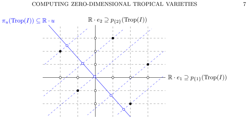
The load-bearing object is the slim unimodular transformation: a torus automorphism that replaces one variable $x_\ell$ by $x_\ell$ times a Laurent monomial in the remaining variables, with exponent vector having one $-1$ and all other entries nonnegative. Its associated linear functional $\pi_u$ projects $\mathbb{R}^n$ onto one coordinate in a direction that can separate finitely many points. The key identity (Lemma 3.2) is $\pi_u(\operatorname{Trop}(I)) = \operatorname{Trop}(\phi_u(I) \cap K[x_\ell^{\pm}])$, which turns a projection of the tropical variety into a univariate tropical variety computable from the Newton polygon of a minimal polynomial. A companion algorithm updates a lex Gröbner basis in shape position to the transformed basis in $O(d^2 \sum (1+\log u_i))$ field operations, by inverting and multiplying univariate polynomials modulo $f_n$. The gluing step then filters the candidate set $w \in \mathbb{R}^A$ whose coordinate projections are already known by testing whether $\pi_u(w)$ lies in the univariate tropical variety.

What would settle it

Compute Trop(I) for a zero-dimensional ideal in shape position over the 2-adic numbers by Algorithm 4.2 and independently by p-adic root approximation, comparing point sets with multiplicities; any mismatch would refute the correctness claim. A sharper test is to search for an ideal whose smallest injective slope $m$ exceeds $\binom{d^2}{2}$, which would contradict Lemma 7.4.

Watch

Extended reading notes

Core claim

The central claim is that Trop(I) for a zero-dimensional ideal $I \subseteq K[x^{\pm}]$ is completely determined by a small collection of univariate tropical varieties, and that these data can be assembled exactly. The paper shows that for a slim unimodular transformation $\phi_u$, the image of Trop(I) under the linear functional $\pi_u$ equals the tropical variety of the elimination ideal $\phi_u(I) \cap K[x_\ell^{\pm}]$, a univariate object read off from a Newton polygon. Using this identity, Algorithm 4.1 merges any two known projections into a larger projection by picking $u$ so that $\pi_u$ separates the finite candidate set, and Algorithm 4.2 repeatedly applies this merge until the full set is obtained. Theorem 7.6 states that the sequential strategy uses $O(n d^2 \log d \log \log d)$ coefficient-field operations and $O(n d^4)$ rational operations, given a reduced lex Gröbner basis of shape position and a valuation $\nu(K^*) \subseteq \mathbb{Q}$. The authors also argue that plugging this algorithm into tropical-link computations makes link computation polynomial-time on average, so that the Gröbner walk dominates in positive dimension.

Load-bearing premise

The polynomial-time guarantee assumes the field's valuation takes only rational values and that a reduced lex Gröbner basis in shape position is supplied; if either fails, the stated complexity bound is not established.

Editorial extensions

If this is right

A zero-dimensional tropical variety can be computed exactly from the coordinate-axis tropical projections, with no need to solve polynomial systems or approximate roots in the valuation topology.
For an ideal of degree $d$ presented by a shape-position lex Gröbner basis, the sequential gluing strategy keeps every candidate set at size at most $d^2$, so both work and memory stay polynomial in $d$ and $n$.
The complexity bound makes the computation of tropical links, the local step that guides the Gröbner walk in existing tropical-variety software, a polynomial-time subtask on average for zero-dimensional links.
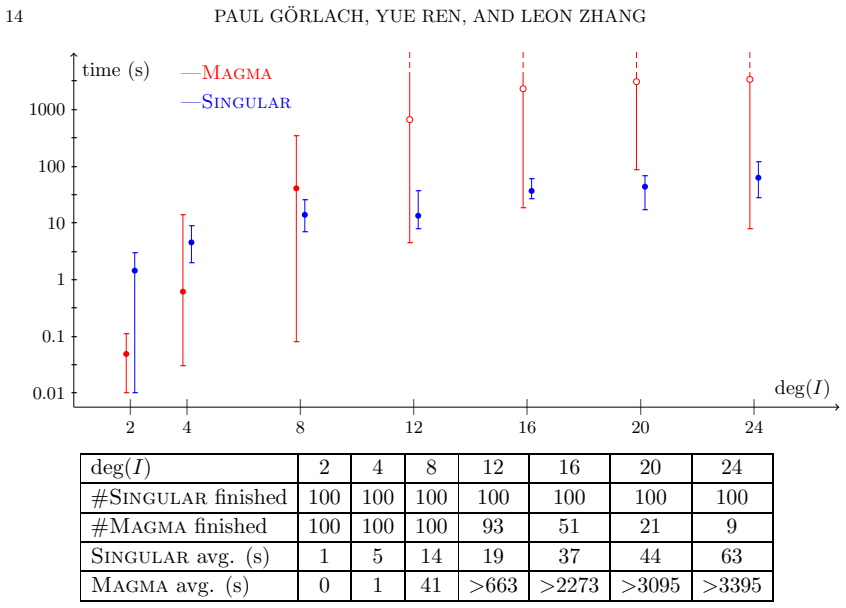
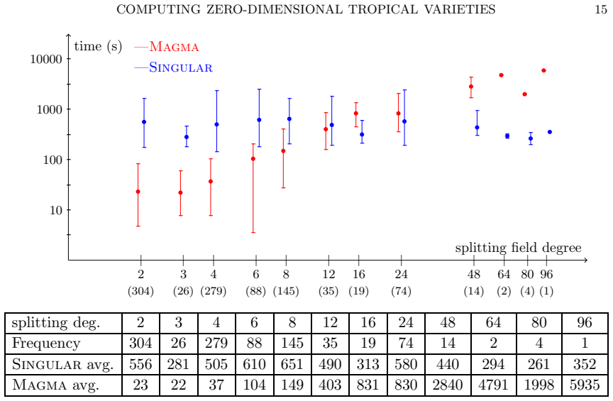
In practice, the projection method scales with degree rather than with the size of the splitting field, which is what slows down p-adic root-approximation baselines.

Reading between the lines

Editorial extensions of the paper, not claims the author makes directly.

The projection-and-gluing paradigm suggests that zero-dimensional tropical computation is essentially univariate: the multivariate structure enters only through the choice of finitely many injective linear functionals, so randomized or heuristic choices of $u$ could reduce the exact rational-operation cost.
If link computation really becomes polynomial-time, further progress on positive-dimensional tropical varieties will depend mainly on Gröbner basis computation and the Gröbner walk, not on tropical-specific elimination.
The same gluing scheme might extend to positive-dimensional ideals if the finite candidate set is replaced by a polyhedral candidate, offering a route to positive-dimensional tropical varieties without traversing the full Gröbner complex.

Share X Bluesky LinkedIn Reddit HN

Signed reviews

No signed human review yet.

Editorial analysis

A structured set of objections, weighed in public.

Desk editor's note, referee report, and a circularity audit.

Desk Editor's Note

read the letter

Here's the short version: the paper's main algorithm is real, the main theorem is proved for the sequential strategy, and the implementation's default overlap strategy is not covered by that theorem. The positive-dimensional remark is a heuristic extrapolation. None of this sinks the paper, but the abstract should be read with that caveat.

What's actually new: the slim unimodular transformations of lex Gröbner bases, and the gluing algorithm that reconstructs a zero-dimensional tropical variety from coordinate projections. Given a reduced lex Gröbner basis in shape position, the algorithm runs in polynomial arithmetic operations in the degree and dimension — O(n d^2 log d log log d) over K, O(n d^4) over Q — assuming rational valuations. That's a genuine improvement over Chan's elimination and Hofmann-Ren's root approximation. The correctness proofs (Lemmas 3.2, 3.3 and the algorithm correctness) look clean. The timings against Magma are believable and show the method scales better at higher degree.

Soft spots, in proportion: (1) Theorem 7.6 only covers the sequential gluing strategy. Section 5.4 says the implementation used for the timings uses the overlap strategy, for which no complexity bound is proved. The paper is not hiding this, but the abstract's 'polynomial number of arithmetic operations' without qualification is likely to be read as covering the implemented algorithm. It would help to either extend the analysis to overlap or qualify the abstract. (2) Remark 7.7, that tropical link computation is dominated by the Gröbner walk, is an argument based on average-case bounds for zero-dimensional Gröbner bases. It is clearly labeled as an argument, so I wouldn't call it a fatal flaw, but it's not a theorem. (3) The algorithm assumes shape position and a lex Gröbner basis input; the complexity of getting to that state is not part of the analysis. That's standard for this kind of paper.

The citation pattern looks reasonable — Chan, Hofmann-Ren, and the standard tropical geometry references are cited appropriately. Code and data are announced but not independently verifiable from the preprint.

For whom: computational tropical geometers and people using Singular to compute tropical varieties. It deserves a serious referee; I'd send it to a journal like JSC or MCOM. The referee should push for a clear statement of which strategy the complexity theorem covers and whether the implementation's strategy can be brought under the same proof.

Referee Report

2 major / 5 minor

Summary. The paper presents an algorithm for computing the tropical variety of a zero-dimensional ideal from a lexicographical Gröbner basis in shape position. The method rests on 'slim' unimodular transformations, which map the given Gröbner basis to one for the transformed ideal, and then reduce the computation to univariate minimal polynomials and Newton polygons. Projections of the tropical variety onto coordinate subspaces are computed separately and then glued via Algorithm 4.1, with Algorithm 4.2 assembling the full tropical variety. The authors prove correctness of these algorithms, give a complexity analysis for the sequential gluing strategy, describe a Singular implementation, compare timings with a p-adic root-approximation approach in Magma, and discuss implications for computing positive-dimensional tropical links.

Significance. If the proof is completed, this is a valuable contribution: it gives a polynomial bound in the degree and ambient dimension for computing zero-dimensional tropical varieties from a Gröbner basis, avoiding both elimination and root approximation to unknown precision. The paper ships an implementation and reproducible benchmark data, and the honeycomb-cubic example is a meaningful stress test. The explicit complexity theorem for the sequential strategy, the exact minimal-polynomial/Newton-polygon steps, and the preservation of shape position and saturation are all concrete strengths that make the central idea credible and potentially useful for subsequent work on tropical links.

major comments (2)

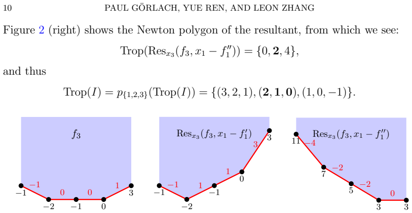
[Section 7, Proposition 7.5] The proof of Proposition 7.5 states that ϕ_w(I) = ϕ_u(ϕ_v(I)) for u := m e_k − e_ℓ. This equality does not hold: for two slim transformations v and u concentrated at the same coordinate ℓ, one computes (ϕ_u∘ϕ_v)(x_ℓ) = x_ℓ · ∏_{i≠ℓ} x_i^{v_i-u_i}, whereas ϕ_w(x_ℓ) = x_ℓ^{-1} · ∏_{i≠ℓ} x_i^{w_i}. In particular, the exponents of x_ℓ differ by sign. Thus Algorithm 3.4 applied to u and a Gröbner basis of ϕ_v(I) produces a Gröbner basis of the composite ideal, not of ϕ_w(I). The intended invariant should be formulated on the level of elimination ideals: applying Algorithm 3.4 to u and the known basis of ϕ_v(I) yields an ideal whose elimination ideal in x_ℓ has tropical variety π_{v+m e_k}(Trop(I)), which is exactly what the gluing step requires. This repair is localized and does not change the stated operation counts, but Theorem 7.6 relies on this proposition, so the proof as written is incomplete. Additionally, for k=2 the induction assumption 'known from a previous call of Algorithm 4.1' is not satisfied; an initial slim transformation and its Gröbner basis must be supplied or computed, adding an O(d^2) cost that is within the claimed bound.
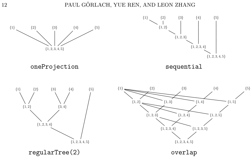
[Sections 5.4, 6, and Theorem 7.6] The complexity guarantee is proved only for the sequential gluing strategy, whereas the implementation and the timings in Section 6 use the overlap strategy. For overlap, the candidate set T in Algorithm 4.1 is a relation with equality constraints on a common prefix, not a Cartesian product, so Lemma 7.4 does not directly apply; no analogue is proved bounding the size of the separating integer or the cost of finding it. Consequently, the abstract's claim that 'our algorithm requires only a polynomial number of arithmetic operations' is not supported for the strategy actually used in the benchmarks. The authors should either prove a complexity bound for the overlap strategy or explicitly restrict the polynomial-complexity claim to the sequential strategy and state that the implemented default strategy is not covered.

minor comments (5)

[Lemma 3.2] The proof uses the equality p_ℓ(Trop(J)) = Trop(J ∩ K[x_ℓ^±]) for zero-dimensional ideals without comment; since this equality is not valid for arbitrary ideals, a short justification in this setting would improve readability.
[Example 4.3] The notation ϕ_{(−1,3)}(I) omits the third coordinate of the transformation; writing ϕ_{(−1,3,0)}(I) would avoid confusion.
[Convention 7.1 / Theorem 7.6] The assumption ν(K*) ⊆ Q is explicit in Section 7 but should be restated in the abstract or in the statement of Theorem 7.6 so that the polynomial bound is not over-read to arbitrary valued fields.
[Remark 7.7] The extrapolation to positive-dimensional tropical links relies on the heuristic claim that zero-dimensional Gröbner bases can be computed in average polynomial time; please label this as experimental/heuristic and distinguish it from the proved Theorem 7.6.
[Throughout] The text contains residual LaTeX markup artifacts such as '/lessnotequal' and 'bracehtipupleft' in the rendering; these should be cleaned in the journal version.

Circularity Check

0 steps flagged · score 0.0 of 10

No significant circularity: the algorithm derives tropical points from exact Gröbner-basis data and univariate elimination, with no fitted quantity renamed as a prediction.

full rationale

The paper's derivation chain is self-contained in the relevant sense: Algorithm 4.2 takes as input a reduced lexicographical Gröbner basis in shape position, computes univariate tropical varieties from Newton polygons of eliminants, and reconstructs Trop(I) by gluing projections. The correctness proofs of Algorithms 4.1 and 4.2 use Lemma 3.2 (πu(Trop(I)) = Trop(ϕu(I) ∩ K[xℓ^±])) and the well-known univariate Newton-polygon fact, neither of which is defined in terms of the target output. Algorithm 3.4 transforms the Gröbner basis by explicit polynomial arithmetic, and no parameter is fitted to a subset of the tropical data and then reported as a prediction. The complexity statement Theorem 7.6 is honestly scoped to the sequential strategy; Section 5.4 states that the overlap strategy is used in the timings, and the paper gives no analogue of Lemma 7.4 or Proposition 7.5 for the overlap candidate relation. This is a scope-of-guarantee mismatch rather than a circular derivation. The references to [Cha13] and [HR18] are contextual or comparative, not load-bearing for the main theorem, and the standard complexity facts are cited from [GG13]. Remark 7.7 explicitly presents the positive-dimensional complexity claim as an argument based on average-case Gröbner basis results, not as a theorem forced by the paper's own equations. No self-definitional step, fitted-input-called-prediction, or ansatz-smuggled-via-citation pattern is present.

Assumptions & free parameters 0 free parameters · 5 assumptions · 0 invented entities

The paper introduces no fitted constants. It relies on standard results in tropical geometry, Gröbner basis theory, and polynomial arithmetic, plus explicit domain assumptions: the field has a nontrivial valuation, zero-dimensional ideals are in shape position, and the value group is rational for the complexity claims. No new physical or algebraic entities are postulated.

assumptions (5)

domain assumption K has a non-trivial valuation ν: K^* → R
Convention 2.1 fixes the setting; the definition of tropical variety (Definition 2.2) requires a valuation.
domain assumption The value group satisfies ν(K^*) ⊆ Q for the complexity analysis
Convention 7.1 restricts to rational valuations so Trop(I) ⊆ Q^n and the gluing search in Lemma 7.4 runs in rational arithmetic.
domain assumption The input is a zero-dimensional ideal in shape position with a reduced lex Gröbner basis
Algorithm 4.2 takes G = {fn, x_{n-1}-f_{n-1}, ..., x_1-f_1}; Lemma 2.5 shows shape position is generically reachable, but the complexity theorem counts from this input onward.
standard math Standard complexity bounds for univariate polynomial arithmetic over K
Proposition 7.2 quotes von zur Gathen and Gerhard (GG13) for O(d^2) operations in K[z]/(f) and O(d^2 log d log log d) for minimal polynomials.
standard math The algebraic closure of the completion of K carries a unique extension of the valuation
Definition 2.2 takes solutions in the algebraic closure of the completion; the uniqueness is a standard fact from valuation theory.

how reviews work

0 comments

Cite this review

Pith. "Pith review of Computing zero-dimensional tropical varieties via projections." pith.science (2026). https://pith.science/paper/7Q3KKZVS

@misc{pith2026190803486,
  author       = {Pith},
  title        = {Pith review of: Computing zero-dimensional tropical varieties via projections},
  year         = {2026},
  howpublished = {\url{https://pith.science/paper/7Q3KKZVS}},
  note         = {Machine review of arXiv:1908.03486}
}

read the original abstract

We present an algorithm for computing zero-dimensional tropical varieties using projections. Our main tools are fast unimodular transforms of lexicographical Gr\"obner bases. We prove that our algorithm requires only a polynomial number of arithmetic operations if given a Gr\"obner basis, and we demonstrate that our implementation compares favourably to other existing implementations. Applying it to the computation of general positive-dimensional tropical varieties, we argue that the complexity for calculating tropical links is dominated by the complexity of the Gr\"obner walk.

Figures

Figures reproduced from arXiv: 1908.03486 by the authors.

**Figure 1.** Computing zero-dimensional tropical varieties via projections. Algorithm 4.1 (gluing projections) Input: (G, pA1 (Trop(I)), . . . , pAk (Trop(I))), where • G is the lexicographical Gr¨obner basis of a zero-dimensional ideal I ⊆ K[x ±] in shape position as in (SP), • A1, . . . , Ak ⊆ {1, . . . , n} are non-empty sets. Output: pA(Trop(I)) ⊆ R A, where A := A1 ∪ . . . ∪ Ak. 1: Construct the candidate set T := n w ∈ R A… view at source ↗

**Figure 2.** (right) shows the Newton polygon of the resultant, from which we see: Trop(Resx3 (f3, x1 − f ′′ 1 )) = {0, 2, 4}, and thus Trop(I) = p{1,2,3}(Trop(I)) = {(3, 2, 1),(2, 1, 0),(1, 0, −1)}. −1 0 0 1 −1 −2 −1 0 3 f3 −1 1 1 3 −1 −2 −1 0 3 Resx3 (f3, x1 − f ′ 1 ) −4 −2 −2 0 11 7 5 3 3 Resx3 (f3, x1 − f ′′ 1 ) [PITH_FULL_IMAGE:figures/full_fig_p010_2.png] view at source ↗

**Figure 3.** Visualisation of different gluing strategies. oneProjection: Only a single iteration of the while loop, in which we pick k = n and Ai = {i} for i = 1, . . . , n. sequential: n − 1 iterations of the while loop, during which we pick k = 2 and A1 = {1, . . . , i} and A2 = {i + 1} in the i-th iteration. regularTree(k): n − 1 iterations of the while loop, which can be partially run in parallel in ⌈logk n⌉ batches. In eac… view at source ↗

Figures from the paper (2 more)

**Figure 4.** Figure 4: Timings for the randomly generated ideals in shape position. 6.2. Tropical lines on a random honeycomb cubic. Let V (f) ⊆ P 3 be a smooth cubic surface. In [PV19], it is shown that Trop(f) ⊆ R 3 may contain infinitely many tropical lines. However, for general f whose c…

**Figure 5.** Figure 5: Timings for the 27 tropical lines on a tropical honeycomb cubic. 7. Complexity In this section, we bound the complexity for computing a zero-dimensional tropical variety from a given Gr¨obner basis using Algorithm 4.2 with the sequential strategy. We show that the num…

Discussion (0). Continue with ORCID to comment.

Forward citations

Cited by 1 Pith paper

Reviewed papers in the Pith corpus that reference this work. Sorted by Pith novelty score. Full citation record

An Octanomial Model for Cubic Surfaces
math.AG 2019-08 conditional novelty 6.0 of 10

A new sparse octanomial normal form for cubic surfaces is defined, and p-adic tropical smoothness in this family forces the 27 lines to be distinct and defined over Q_p.

Reference graph

Works this paper leans on

11 extracted references · 9 canonical work pages · cited by 1 Pith paper

[1]

Log-barrier inte- rior point methods are not strongly polynomial

[ABGJ18] X. Allamigeon, P. Benchimol, S. Gaubert, and M. Jos wig. “Log-barrier inte- rior point methods are not strongly polynomial”. In: SIAM J. Appl. Algebra Geom. 2.1 (2018), pp. 140–178. [AK06] F. Ardila and C. J. Klivans. “The Bergman complex of a m atroid and phy- logenetic trees”. In: J. Combin. Theory Ser. B 96.1 (2006), pp. 38–49. [BK19] E. Baldw...

work page 2018
[7]

Progr. Math. Birkh¨ auser Boston, Boston, MA, 1991 , pp. 217–225. [LMY18] B. Lin, A. Monod, and R. Yoshida. Tropical Foundations for Probability & Statistics on Phylogenetic Tree Space . eprint: arXiv:1805.12400

arXiv 1991
[14]

The discriminant of a cubic surface

Algorithms and Computation in Mathematics. Foundations, a lgorithms, and applications. Springer-Verlag, Berlin, 2005, pp. xiv+425 . [EJ12] A.-S. Elsenhans and J. Jahnel. “The discriminant of a cubic surface”. In: Geom. Dedicata 159 (2012), pp. 29–40. [FGLM93] J. C. Faug` ere, P. Gianni, D. Lazard, and T. Mora. “E ﬃcient computation of zero-dimensional Gr¨...

work page 2012
[29]

Finiteness of spatial cent ral conﬁgurations in the ﬁve-body problem

DMV Sem. Birkh¨ auser, Basel, 2000, pp. 43–73. [GP02] G.-M. Greuel and G. Pﬁster. A Singular introduction to commutative al- gebra. With contributions by Olaf Bachmann, Christoph Lossen and Hans Sch¨ onemann. Springer-Verlag, Berlin, 2002, pp. xviii+588. [HJ11] M. Hampton and A. Jensen. “Finiteness of spatial cent ral conﬁgurations in the ﬁve-body problem...

work page 2011
[73]

The Magma alge bra system. I. The user language

[BCP97] W. Bosma, J. Cannon, and C. Playoust. “The Magma alge bra system. I. The user language”. In: J. Symbolic Comput. 24.3-4 (1997). Computational algebra and number theory (London, 1993), pp. 235–265. [Cha13] A. Chan. “Gr¨ obner bases over ﬁelds with valuation a nd tropical curves by coordinate projections”. PhD thesis. University of Warwic k,

work page 1997
[94]

On the complexity of zer o-dimensional algebraic systems

Progr. Math. Birkh¨ auser Boston, Boston, MA, 1991, pp. 227–234. [LL91] Y. N. Lakshman and D. Lazard. “On the complexity of zer o-dimensional algebraic systems”. In: Eﬀective methods in algebraic geometry (Castiglion- cello,

work page 1991
[97]

Product-Mix Auctions and Tropical Geometry

CBMS Re- gional Conference Series in Mathematics. Published for the Conference Board of the Mathematical Sciences, Washington, DC; by the Americ an Mathemat- ical Society, Providence, RI, 2002, pp. viii+152. [TY15] N. M. Tran and J. Yu. Product-Mix Auctions and Tropical Geometry. eprint: arXiv:1505.05737

work page Pith review arXiv 2002
[161]

Enumerative tropical algebraic geo metry in R2

Graduate Studies in Mathematics. American Mathematical So ciety, Provi- dence, RI, 2015, pp. xii+363. [Mik05] G. Mikhalkin. “Enumerative tropical algebraic geo metry in R2”. In: J. Amer. Math. Soc. 18.2 (2005), pp. 313–377. 20 REFERENCES [Neu99] J. Neukirch. Algebraic number theory . Vol

work page 2005

Show all 11 references

[185]

Springer, Ne w York, 2005, pp

Graduate Texts in Mathematics. Springer, Ne w York, 2005, pp. xii+572. [DGPS19] W. Decker, G.-M. Greuel, G. Pﬁster, and H. Sch¨ onem ann. Singular 4-1-2 — A computer algebra system for polynomial computations . http://www.s ingular.uni-kl.de

2005
[1999]

Panizzut and M

[PV19] M. Panizzut and M. D. Vigeland. Tropical Lines on Cubic Surfaces . eprint: arXiv:0708.3847v2

arXiv
[2019]

The tropical Grassmanni an

[SS04] D. Speyer and B. Sturmfels. “The tropical Grassmanni an”. In: Adv. Geom. 4.3 (2004), pp. 389–411. [Ste19] A. Steenpass. modular.lib. A Singular 4-1-2 library for modular tech- niques

2004

Pith tools

Reviewed August 14, 2026 · model on record in the stance chip above.

[1] [1]

Log-barrier inte- rior point methods are not strongly polynomial

[ABGJ18] X. Allamigeon, P. Benchimol, S. Gaubert, and M. Jos wig. “Log-barrier inte- rior point methods are not strongly polynomial”. In: SIAM J. Appl. Algebra Geom. 2.1 (2018), pp. 140–178. [AK06] F. Ardila and C. J. Klivans. “The Bergman complex of a m atroid and phy- logenetic trees”. In: J. Combin. Theory Ser. B 96.1 (2006), pp. 38–49. [BK19] E. Baldw...

work page 2018

[2] [7]

Progr. Math. Birkh¨ auser Boston, Boston, MA, 1991 , pp. 217–225. [LMY18] B. Lin, A. Monod, and R. Yoshida. Tropical Foundations for Probability & Statistics on Phylogenetic Tree Space . eprint: arXiv:1805.12400

arXiv 1991

[3] [14]

The discriminant of a cubic surface

Algorithms and Computation in Mathematics. Foundations, a lgorithms, and applications. Springer-Verlag, Berlin, 2005, pp. xiv+425 . [EJ12] A.-S. Elsenhans and J. Jahnel. “The discriminant of a cubic surface”. In: Geom. Dedicata 159 (2012), pp. 29–40. [FGLM93] J. C. Faug` ere, P. Gianni, D. Lazard, and T. Mora. “E ﬃcient computation of zero-dimensional Gr¨...

work page 2012

[4] [29]

Finiteness of spatial cent ral conﬁgurations in the ﬁve-body problem

DMV Sem. Birkh¨ auser, Basel, 2000, pp. 43–73. [GP02] G.-M. Greuel and G. Pﬁster. A Singular introduction to commutative al- gebra. With contributions by Olaf Bachmann, Christoph Lossen and Hans Sch¨ onemann. Springer-Verlag, Berlin, 2002, pp. xviii+588. [HJ11] M. Hampton and A. Jensen. “Finiteness of spatial cent ral conﬁgurations in the ﬁve-body problem...

work page 2011

[5] [73]

The Magma alge bra system. I. The user language

[BCP97] W. Bosma, J. Cannon, and C. Playoust. “The Magma alge bra system. I. The user language”. In: J. Symbolic Comput. 24.3-4 (1997). Computational algebra and number theory (London, 1993), pp. 235–265. [Cha13] A. Chan. “Gr¨ obner bases over ﬁelds with valuation a nd tropical curves by coordinate projections”. PhD thesis. University of Warwic k,

work page 1997

[6] [94]

On the complexity of zer o-dimensional algebraic systems

Progr. Math. Birkh¨ auser Boston, Boston, MA, 1991, pp. 227–234. [LL91] Y. N. Lakshman and D. Lazard. “On the complexity of zer o-dimensional algebraic systems”. In: Eﬀective methods in algebraic geometry (Castiglion- cello,

work page 1991

[7] [97]

Product-Mix Auctions and Tropical Geometry

CBMS Re- gional Conference Series in Mathematics. Published for the Conference Board of the Mathematical Sciences, Washington, DC; by the Americ an Mathemat- ical Society, Providence, RI, 2002, pp. viii+152. [TY15] N. M. Tran and J. Yu. Product-Mix Auctions and Tropical Geometry. eprint: arXiv:1505.05737

work page Pith review arXiv 2002

[8] [161]

Enumerative tropical algebraic geo metry in R2

Graduate Studies in Mathematics. American Mathematical So ciety, Provi- dence, RI, 2015, pp. xii+363. [Mik05] G. Mikhalkin. “Enumerative tropical algebraic geo metry in R2”. In: J. Amer. Math. Soc. 18.2 (2005), pp. 313–377. 20 REFERENCES [Neu99] J. Neukirch. Algebraic number theory . Vol

work page 2005