REVIEW 3 major objections 5 minor 36 references
Improved GM(1,1) model based on Simpson formula and its applications
T0 review · 3 major / 5 minor · reviewed 2026-08-14 · deepseek-v4-flash
Pith's one-line read A discrete Simpson-formula grey model reproduces exponential sequences exactly and beats three standard grey models on real data.
desk verdict A modest but genuine theoretical fix for GM(1,1) with Simpson background value; the 'outperforms' claim is not supported by the tiny empirical differences. read the letter →
The pith
A machine-rendered reading of the paper's core claim, the machinery that carries it, and where it could break.
The reading
What carries the argument
The central object is the Simpson background value $z^{(1)}(k)=\frac{x^{(1)}(k-1)+4x^{(1)}(k)+x^{(1)}(k+1)}{3}$, used to discretize the whitening equation $\frac{dx^{(1)}(t)}{dt}+ax^{(1)}(t)=b$ over the interval $[k-1,k+1]$. This produces the second-order difference equation $(a+3)x^{(1)}(k+1)+4ax^{(1)}(k)+(a-3)x^{(1)}(k-1)-6b=0$, which the paper rewrites as a first-order linear difference equation in $x^{(1)}(k+1)-wx^{(1)}(k)$, with $w=\frac{\sqrt{3a^2+9}-2a}{a+3}$. The time response (Eq. 14) is the exact solution of this difference equation, not a sampled exponential, and that exactness is what makes the model unbiased for homogeneous exponential sequences and free of the parameter-dependent error of the continuous GMSC(1,1).
What would settle it
Take the sequence $x^{(0)}(k)=rq^k$ with $q=2.25$ and $r=0.05$ as in Table 2, fit GMSD(1,1), and verify that the restored values equal $rq^k$ to machine precision. Then repeat the comparison on a non-exponential series, such as a linear or quadratic trend or a geometric series with additive noise, and check whether GMSD(1,1) still has the lowest rolling MAPE; if its advantage does not persist, the practical superiority claim is limited to near-exponential data.
Extended reading notes
Core claim
The paper's central discovery is that replacing the trapezoidal background value of GM(1,1) with the Simpson-rule value, and crucially using the exact solution of the resulting difference equation as the time response, yields a discrete model that is unbiased for homogeneous exponential sequences. In Section 3.4, for $X^{(0)}(k)=rq^k$, the least-squares estimates of $a$ and $b$ reduce to $3(1-q^2)/(1+4q+q^2)$ and $3rq(1+q)/(1+4q+q^2)$, which forces $w=q$; substituting into the restored-value formula gives $\hat{x}^{(0)}(k+1)=x^{(0)}(k+1)$, so simulation and prediction coincide with the true series. The paper also shows that the continuous Simpson-based model GMSC(1,1) does not share this property: its exponential time response satisfies the discretized equation only when $|a|$ is small, and its errors on exact exponential data grow with $|a|$.
Load-bearing premise
The exactness result assumes the data are a pure geometric sequence $rq^k$, and the real-data advantage is demonstrated on only three data sets, so the general claim of superior forecasting rests on those examples.
Editorial extensions
If this is right
- For exact homogeneous exponential data, GMSD(1,1) achieves simulation and prediction errors at the $10^{-13}$ percent level, effectively machine precision, while GMSC(1,1) errors grow with $|a|$.
- In the electricity consumption example, GMSD(1,1) has the lowest prediction MAPE (3.2669%) among the four models, ahead of GMSC(1,1) (3.5137%), GM(1,1) (5.0428%), and DGM(1,1) (5.1811%).
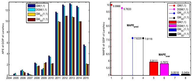
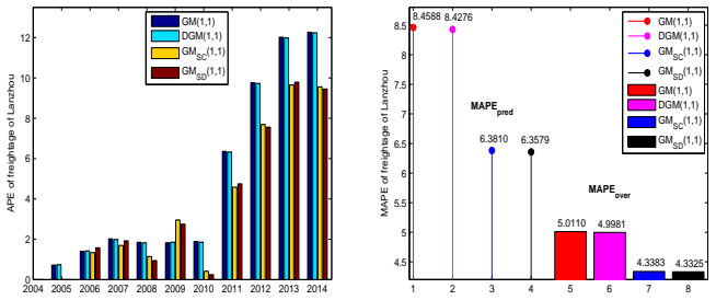
- In the Lanzhou GDP application, GMSD(1,1) has the lowest prediction MAPE (7.6118%) and overall MAPE (5.0454%); in the freightage application, the corresponding values are 6.3579% and 4.3325%.
- Because the time response is the exact solution of the model's own difference equation, the model's accuracy does not degrade for large values of the system parameter $a$, a limitation of the continuous Simpson model.
- The paper's closing remark proposes that the same discretization idea can be carried over to other grey models such as GM(1,n) and GMC(1,n).
Reading between the lines
- The unbiasedness theorem is exact only for pure geometric sequences; for real series the reported advantage is empirical, so a natural next test is whether the model keeps its edge on noisy or trended data.
- Because Simpson's rule uses three consecutive accumulated values, the model effectively incorporates second-order information; this suggests a family of higher-order quadrature grey models, and one could test whether Newton-Cotes formulas of higher order preserve or improve the unbiasedness property.
- The paper's suggestion to extend the idea to GM(1,n) and GMC(1,n) could be made concrete by checking whether the exact-solution construction removes parameter-dependence in multi-variable grey models as it does here.
Signed reviews
Editorial analysis
A structured set of objections, weighed in public.
Referee Report
Summary. The paper proposes a discrete grey model, GMSD(1,1), whose background value is constructed with the Simpson numerical integration formula, and whose time response function is the exact solution of the resulting second-order difference equation. The parameters are estimated by least squares, the discrete model is contrasted with the continuous GMSC(1,1) model, and a proof is given that GMSD(1,1) is unbiased for homogeneous exponential sequences. Numerical examples compare GMSD(1,1) with GM(1,1), DGM(1,1), and GMSC(1,1) on a synthetic exponential sequence and on three real datasets (China's electricity consumption, Lanzhou's GDP, and Lanzhou's freightage), with the empirical sections claiming that GMSD(1,1) provides the most accurate predictions.
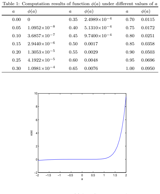
Significance. The theoretical core of the paper is sound and useful: the discrete time response is internally consistent with the fitted difference equation, the unbiasedness theorem in Section 3.4 is a genuine algebraic result, and Section 3.3 gives a clean diagnostic, the function phi(a), showing why the continuous GMSC(1,1) model is inconsistent when |a| is not small. These contributions are modest but real within the grey-systems literature. The main weakness is that the paper's headline practical claim, that GMSD(1,1) 'outperforms' the other three models, rests on very small point estimates of MAPE on short test sets without any uncertainty quantification. The absence of code and data also makes the numerical comparisons difficult to verify. If the empirical claims are strengthened or suitably weakened, the paper would be a solid contribution to specialized journals in this area.
major comments (3)
- [Section 5; Tables 4-7] The central empirical claim that GMSD(1,1) outperforms GM(1,1), DGM(1,1), and GMSC(1,1) is not supported by the evidence as presented. The reported prediction advantages are extremely small: in Table 5, MAPE_pred is 7.6118% versus 7.6220% for GMSC; in Table 7, it is 6.3579% versus 6.3810%; and in Table 3, it is 3.2669% versus 3.5137% on only three test observations. No confidence intervals, significance tests, or sensitivity analyses are given, and the in-sample MAPE_simu of GMSD(1,1) is the worst among all four models in every application (e.g., Table 3: 1.7387% versus 1.5675% for GM(1,1)). These differences are within the noise of a handful of data points. The authors should either provide proper uncertainty quantification and a test for equality of forecast errors, or substantially weaken the concluding statement to say that GMSD(1,1) performs comparably on these particular datasets rather than claiming general superiority.
- [Section 3.4; Eq. (22)] The unbiasedness proof rests on the closed-form least-squares solution stated in Eq. (22), but the derivation is presented with the phrase 'After some calculations' and the algebra is not shown. This is the load-bearing step that identifies the estimated parameters with the values 3(1-q^2)/(1+4q+q^2) and 3rq(1+q)/(1+4q+q^2). The authors should provide the full derivation, including the computation of B^T B and its inverse, and state the conditions under which the inverse exists (for instance, the number of fitting points n and the range of q). Without this, a central result of the paper is not verifiable from the manuscript text.
- [Section 3.3; Eq. (18); Tables 3, 4, 6] The numerical implementation of the benchmark models is not transparent. Equation (18) defines the GMSC time response using x(0)(1) as the initial value, and in general this does not reproduce x(0)(2) from the raw data; nevertheless, the GMSC columns in Tables 3, 4, and 6 show exact agreement with the actual value at k=2 (e.g., 28588.0000, 567.0400, and 5973.0000). At the same time, the GMSD response in Eq. (14) uses x(1)(1) and x(1)(2) as initial conditions, so by construction it interpolates the first two original data points. The authors should specify the exact initial-condition convention and the fitted time index set for each of the four models, and state explicitly whether any fitted values are set equal to the observed data by construction. Without this information, the reported advantages could be artifacts of different initialization schemes rather than of the Simpson-based background value.
minor comments (5)
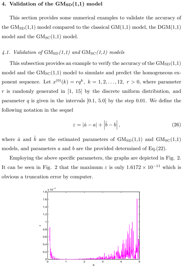
- [Section 4.1; Eq. (26)] The text says 'parameters a and b are the provided determined of Eq.(22)'; this should be reworded as 'the provided values determined by Eq. (22)'. Also, Figure 2 depends on r, which is described only as randomly generated in [1,15]; please report a seed or the exact generated values so that the figure is reproducible.
- [Introduction, Section 3] The Introduction states that the paper 'study the forecast stability problem' of the discrete GMSD(1,1) model, but no dedicated stability analysis appears in Section 3 or elsewhere. Section 3.3 discusses parameter dependence and inconsistency of GMSC(1,1), which is related but not identical to forecast stability; the text should be aligned with what is actually studied.
- [Equations (14)-(15)] The derivation of Eq. (14) is presented for k = 2, 3, ..., n-1, whereas Eq. (15) is stated for k = 1, 2, ..., n-1. Please clarify how the boundary cases k=1 and k=n are defined, since the sums and powers in the formulas involve k-2 and could otherwise be ambiguous.
- [Throughout] There are several typos and formatting inconsistencies, for example 'thw development' in Section 1 and the inconsistent spacing of 'GMSC' and 'GMSD' (e.g., 'GM SC(1,1)' versus 'GMSD(1,1)'). A careful proofreading pass is needed.
- [Numerical reproducibility] No code or data availability statement is provided. Given that the paper makes quantitative comparisons on real datasets, the raw data and the implementation of the four models should be made available, or at least the data should be provided in an appendix, so that the reported MAPE values can be checked.
Circularity Check
No circularity: GMSD(1,1) is derived from a Simpson-rule discretization, its time response solves the fitted difference equation, and the homogeneous-exponential unbiasedness theorem is an algebraic self-consistency result rather than a fitted prediction.
full rationale
I walked the derivation chain: the model is built by integrating the whitening equation over [k-1, k+1] and applying Simpson's rule to obtain Eq. (9)/(10); Eq. (14) is obtained by algebraic iteration of the resulting second-order difference equation; parameters are estimated by ordinary least squares from Eq. (16); and forecasts are evaluated on held-out samples (Tables 3, 4, 6). No step defines the target as an input or fits a parameter to the quantity being predicted. The unbiasedness theorem in Section 3.4 considers exact homogeneous exponential sequences X(0)(k) = r q^k; substituting the exact 1-AGO forms into B and Y gives the closed-form least-squares solution (22), and substituting (22) into the response formula (15) reduces algebraically to x(0)(k+1) = r q^{k+1}. That is a mathematical consistency property of the estimator, not a circular prediction: the conclusion is derived from the model equations and the assumed data-generating form, not assumed as an input. The paper does cite several earlier papers by the same authors (e.g., refs. 15-19, 26, 33, 34), but these appear as background references for grey-model applications and do not carry the derivation, parameter estimation, or unbiasedness proof. No uniqueness theorem from the authors' prior work is invoked, and no ansatz is smuggled in through a self-citation. The empirical claim that GMSD "outperforms" the other models rests on small MAPE differences and a few test points, and the skeptic's point about lack of statistical testing is a legitimate robustness concern; however, that is a correctness/evaluation issue, not circularity. I therefore find no circular step and set the score to 0.
Assumptions & free parameters
free parameters (2)
- a =
dataset-dependent (least squares, Eq. 17)
- b =
dataset-dependent (least squares, Eq. 17)
assumptions (4)
- domain assumption The 1-AGO series x1(k) satisfies the whitening differential equation dx1/dt + a x1 = b.
- domain assumption The Simpson rule gives an adequate approximation of the integral of x1(t) over [k-1, k+1].
- domain assumption The unbiasedness proof assumes the original series is exactly the homogeneous exponential sequence X(0)(k)=r q^k.
- standard math Least squares estimation yields the model parameters a and b from the discretized equation.
Cite this review
Pith. "Pith review of Improved GM(1,1) model based on Simpson formula and its applications." pith.science (2026). https://pith.science/paper/5GQB6UHT
@misc{pith2026190803493,
  author       = {Pith},
  title        = {Pith review of: Improved GM(1,1) model based on Simpson formula and its applications},
  year         = {2026},
  howpublished = {\url{https://pith.science/paper/5GQB6UHT}},
  note         = {Machine review of arXiv:1908.03493}
}
abstract
The classical GM(1,1) model is an efficient tool to {make accurate forecasts} with limited samples. But the accuracy of the GM(1,1) model still needs to be improved. This paper proposes a novel discrete GM(1,1) model, named ${\rm GM_{SD}}$(1,1) model, of which the background value is reconstructed using Simpson formula. The expression of the specific time response function is deduced, and the relationship between our model} and the continuous GM(1,1) model with Simpson formula called ${\rm GM_{SC} }$(1,1) model is systematically discussed. The proposed model is proved to be unbiased to simulate the homogeneous exponent sequence. Further, some numerical examples are given to validate the accuracy of the new ${\rm GM_{SD}}$(1,1) model. Finally, this model is used to predict the Gross Domestic Product and the freightage of Lanzhou, and the results illustrate the ${\rm GM_{SD}}$(1,1) model provides accurate prediction.
Figures
Figures from the paper (1 more)
Reference graph
Works this paper leans on
-
[1]
Deng, Control problems of grey systems, Systems & Contro l Letters 1 (5) (1982) 288–294
J. Deng, Control problems of grey systems, Systems & Contro l Letters 1 (5) (1982) 288–294
work page 1982
-
[2]
Q. Xiao, C. Li, Y. Tang, L. Li, L. Li, A knowledge-deriven method of adap- tively optimiizing process parameters for energy efficient turning, E nergy 166 (2019) 142–156
work page 2019
-
[3]
X. Wu, X. Ding, T. Lu, J. Wang, Topological dynamics of Zadeh’s ex tension on upper semi-continuous fuzzy sets, International Journal of Bifurcation and Chaos 27 (10) (2017) 1–13
work page 2017
-
[4]
P. Du, J. Wang, W. Yang, T. Niu, Multi-step ahead forecasting in e lectrical power system using a hybrid forecasting system, Renewable Energ y 122 (7) (2018) 533–550
work page 2018
-
[5]
M. Ma, W. Cai, Y. Wu, China act on the energy efficiency of civil buildin gs (2008): a decade review, Science of The Total Environment 651 (1 5) (2019) 42–60
work page 2008
-
[6]
Y. Wang, X. Yi, Transient pressure behavior of a fractured ver tical well with a finite-conductivity fracture in triple media carbonate reservoir, Journal of Porous Media 20 (8) (2017) 707–722. 19
work page 2017
-
[7]
Y. Wang, X. Yi, Flow modeling of well test analysis for a multiple-frac tured horizontal well in triple media carbonate reservoir, International Journal of Nonlinear Sciences and Numerical Simulation 19 (5) (2018) 439–45 7
work page 2018
-
[8]
S.-J. Huang, C.-L. Huang, Control of an inverted pendulum using grey prediction model, IEEE Transaction on Industry Application 36 (2) ( 2000) 452–458
work page 2000
Show all 36 references
-
[9]
Chang, H.-C
S.-C. Chang, H.-C. Lai, H.-C. Yu, A variable P value rolling grey forec ast- ing model for Taiwan semiconductor industry production, Technolo gical Forecasting & Social Change 72 (5) (2005) 623–640
2005
-
[10]
Chen, P.-H
C.-I. Chen, P.-H. Hsin, C.-S. Wu, Forecasting Taiwan’s major sto ck in- dices by the Nash nonlinear grey Bernoulli model, Expert Systems wit h Applications 37 (12) (2010) 7557–7562
2010
-
[11]
Z. Wang, Q. Li, L. Pei, Grey forecasting method of quarterly hy dropower production in China based on a data grouping approach, Applied Math e- matical Modelling 51 (11) (2017) 302–316
2017
-
[12]
Z. Wang, H. Zheng, L. Pei, T. Jin, Decomposition of the factors influencing export fluctuation in China’s new energy industry based on a consta nt market share model, Energy Policy 109 (10) (2017) 22–35
2017
-
[13]
B. Zeng, H. Duan, Y. Bai, W. Meng, Forecasting the output of s hale gas in china using an unbiased grey model and weakening buffer operator, Energy 151 (15) (2018) 238–249
2018
-
[14]
W. Zhou, J. He, Generalized GM(1,1) model and its application in fo re- casting of fuel production, Applied mathematical Modelling 37 (9) (2 013) 6234–6243
-
[15]
X. Ma, Z. Liu, The GMC(1, n) model with optimized parameters and its applications, Journal of Grey System 29 (4) (2017) 121–137. 20
2017
-
[16]
W. Wu, X. Ma, B. Zeng, Y. Wang, W. Cai, Application of the novel f rac- tional grey model F AGMO(1,1, k) to predict China’s nuclear energy con- sumption, Energy 165 (2018) 223–234
2018
-
[17]
W. Wu, X. Ma, B. Zeng, Y. Wang, W. Cai, Forecasting short-ter m renew- able energy consumption of China using a novel fractional nonlinear grey Bernoulli model, Renewable Energy 140 (2019) 70–87
2019
-
[18]
X. Ma, M. Xie, W. Wu, X. Wu, B. Zeng, A novel fractional time dela yed grey model with grey wolf optimizer and its applications in forecasting the natural gas and coal sonsumption in Chongqing China, Energy 178 ( 2019) 487–507
2019
-
[19]
W. Wu, X. Ma, Y. Zhang, Y. Wang, X. Wu, Analysis of novel F AGM(1, 1, tα) model to forecast health expenditure of China, Grey Sys- tems: Theory and Application 9 (2) (2019) 232–250
2019
-
[20]
B. Zeng, Y. Tan, H. Xu, J. Quan, L. Wang, X. Zhou, Forecastin g the electricity consumption of commercial sector in Hong Kong using a no vel grey dynamic prediction model, Journal of Grey System 30 (1) (201 8) 157– 172
-
[21]
L. Wu, Y. Gao, Y. Yang, X. Chen, Using a novel multi-variable gre y model to forecast the electricity consumption of Shangdong province in C hina, Energy 157 (15) (2018) 327–335
2018
-
[22]
Zhang, Y
L. Zhang, Y. Zheng, K. Wang, X. Zhang, Y. Zheng, An optimized Nash nonlinear grey Bernoulli model based on particle swarm optimization a nd its application in prediction for the incidence of Hepatitis B in Xinjiang, China, Computers in Biology & Medicine 49 (1) (2014) 67–73
2014
-
[23]
N. Xie, S. Liu, Discrete grey forecasting model and its optimizat ion, Ap- plied Mathematical modelling 33 (2) (2009) 1173–1186. 21
2009
-
[24]
B. Zeng, H. Duan, Y. Zhou, A new multivariable grey prediction mo del with structure compatibility, Applied Mathematical Modelling 75 (2019 ) 385–397
2019
-
[25]
C.-I. Chen, H. Chen, S. Chen, Forecasting of foreign exchang e rates of Taiwan’s major trading partners by novel nonlinear grey Bernoulli m odel NGBM(1, 1), Communications in Nonlinear Science and Numerical Simu- lation 13 (6) (2008) 1194–1204
2008
-
[26]
L. Kong, X. Ma, Comparison study on the nonlinear parameter o ptimiza- tion of nonlinear grey Bernoulli model (NGBM(1,1)), Grey Systems: The- ory and Application 8 (2) (2018) 210–226
2018
-
[27]
L. Pei, Q. Li, Z. Wang, The NLS-based nonlinear grey Bernoulli mo del with an application to employee demand prediction of high-tech enterpris es in China, Grey Systems: Theory and Application 8 (2) (2018) 133–143
2018
-
[28]
Salehi, N
M. Salehi, N. Dehnavi, Audit report forecast: an application of n onlinear grey Bernoulli model, Grey Systems: Theory and Application 8 (3) (2 018) 295–311
-
[29]
D. Q. Truong, K. K. Ahn, An accurate signal estimator using a n ovel smart adaptive grey model SAGM(1,1), Expert Systems with Applications 3 9 (9) (2012) 7611–7620
2012
-
[30]
J. Cui, S. Liu, B. Zeng, N. Xie, A novel grey forecasting model a nd its optimization, Applied Mathematical Modelling 37 (6) (2013) 4399–440 6
2013
-
[31]
B. Zeng, C. Li, Improved multi-variable grey forecasting model with a dynamic background-value coefficient and its application, Computer s & Industrial Engineering 118 (4) (2018) 278–290
2018
-
[32]
M. He, Q. Wang, Constructing the background value for GM(1,1 ) model based on Simpson formula (in chinese), Journal of Quantitative Eco nomics 28 (4) (2011) 101–104. 22
2011
-
[33]
J. Xia, X. Ma, W. Wu, B. Huang, W. Li, Application of a new informat ion priority accumulated grey model with time power to predict short-t erm wind turbine capacity, Journal of Cleaner Production 244 (2020) 1 18573
2020
-
[34]
Ma, A brief introduction to the grey machine learning, Journa l of Grey System 31 (1) (2019) 1–12
X. Ma, A brief introduction to the grey machine learning, Journa l of Grey System 31 (1) (2019) 1–12
2019
-
[35]
Wang, V.-T
C.-N. Wang, V.-T. Phan, An improved nonlinear grey Bernoulli mod el combined with Fourier series, Mathematical Problems in Engineering 2 015 (2015) 1–7
2015
-
[36]
S. Ding, K. W. Hipel, Y. Dang, Forecasting China’s electricity cons umption using a new grey prediction model, Energy 149 (15) (2018) 314–328 . 23
2018
Reviewed August 14, 2026 · model on record in the stance chip above.
Discussion (0). Continue with ORCID to comment.