REVIEW 3 major objections 4 minor 30 references
Enriching MRI mean flow data of inclined jets in crossflow with Large Eddy Simulations
T0 review · 3 major / 4 minor · reviewed 2026-08-14 · deepseek-v4-flash
Pith's one-line read LES enriches MRI flow data with near-wall turbulence
desk verdict A solid, honest method demonstration: validated LES enriches MRI mean fields for an inclined jet in crossflow at three velocity ratios; the main caveat is that near-wall and turbulence quantities are inferred, not directly validated, and the paper knows this. read the letter →
The pith
A machine-rendered reading of the paper's core claim, the machinery that carries it, and where it could break.
The reading
What carries the argument
The central mechanism is the enrichment loop: a fine-mesh LES whose subgrid-scale viscosity is negligible almost everywhere (so it approaches DNS resolution) but which, unlike DNS, is feasible for this geometry; an iterative inlet-condition procedure that tunes a synthetic turbulence generator against hot-wire data until a channel-flow LES matches the measured boundary-layer profile and momentum thickness; and validation against the three-dimensional MRI fields as a whole. The load-bearing identity is the matching of mean velocity and mean concentration between LES and MRV/MRC in the region where both are reliable; agreement there is taken as evidence that the LES is a physically realistic representation of the flow. Quantitative comparisons use integrated quantities, such as the circulation $\Gamma$ of the counter-rotating vortex pair, which are robust to MRI noise and misalignment.
What would settle it
A direct test would measure near-wall velocity and concentration and turbulent fluctuations in the same geometry using an independent technique such as particle image velocimetry or a hot-wire probe, and check whether the LES agrees there as closely as it does for the mean fields away from the wall; systematic disagreement in those quantities while mean fields agree would invalidate the enrichment claim.
Extended reading notes
Core claim
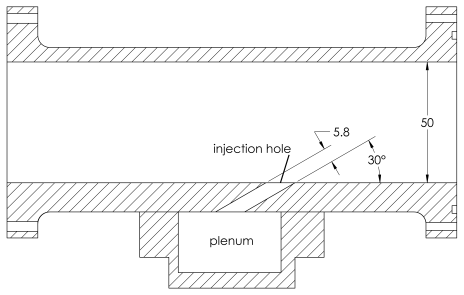
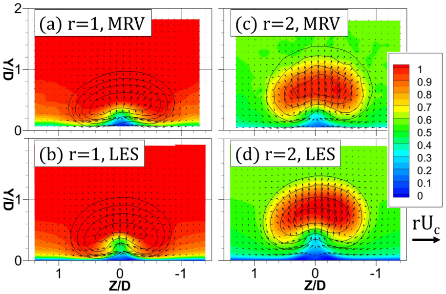
The paper demonstrates that, when the simulation domain and inlet conditions are carefully matched to the experiment, large-eddy simulation reproduces the three-dimensional mean velocity and scalar fields of Magnetic Resonance Velocimetry and Concentration closely enough that the simulation can be trusted where MRI is blind. The validated LES then provides wall concentration (adiabatic effectiveness), in-hole velocity, and turbulent correlations such as Reynolds stresses and scalar fluxes that the experiments cannot measure. The validation is grounded in the full 3D fields rather than single-point comparisons; quantitative metrics like the circulation of the counter-rotating vortex pair are computed independently from both datasets. The simulations reveal that in this geometry the $r=1$ jet reattaches to the wall after injection while $r=1.5$ and $r=2$ remain detached, and that the short $4.1D$ feed hole produces a strongly non-uniform in-hole velocity with a separation bubble, rather than developed pipe flow.
Load-bearing premise
The argument depends on the premise that close agreement in time-averaged velocity and concentration throughout the measured three-dimensional domain implies the simulation is also accurate for near-wall values and turbulent correlations, which are never directly checked against experimental data.
Editorial extensions
If this is right
- For this geometry, the $r=1$ jet detaches briefly and reattaches by $x/D\approx3$, while $r=1.5$ and $r=2$ remain detached, placing the reattachment threshold between $r=1$ and $r=1.5$.
- The LES supplies wall concentration (adiabatic effectiveness) that MRC cannot measure reliably, including the sharp drop after injection and the partial recovery for $r=1$.
- In-hole flow is far from fully developed: a separation bubble on the plenum-side corner causes high axial velocity on the opposite side and secondary flows up to about 20% of the bulk velocity, with little change across $r$ in this range.
- Turbulent statistics from the LES, such as the Reynolds stress $u'v'$ and scalar flux $v'c'$, are now part of the dataset for data-driven turbulence modeling in film cooling flows.
- The counter-rotating vortex pair circulation in the LES follows the experimental trends but is consistently overpredicted, occasionally beyond misalignment-induced uncertainty.
Reading between the lines
- The same enrichment approach could be extended to quantities MRI cannot provide at all, such as wall shear stress or pressure, but each would need its own validation target since mean-field agreement does not guarantee derivative quantities.
- A natural testable extension is to run the same matched LES/MRI protocol with an added planar PIV or LDV check of turbulent statistics in one region; if fluctuations also match, the claim that simulations can be treated as data becomes much stronger.
- The systematic overprediction of circulation suggests the in-hole flow or its coupling to the crossflow differs subtly between simulation and experiment; quantifying the sensitivity to plenum feed details would bound the enrichment's uncertainty.
- The weakly positive $u'v'$ and $v'c'$ under the jet where mean gradients are positive is a concrete signature of gradient-diffusion model failure, giving turbulence modelers a targeted test for new closures.
Editorial analysis
A structured set of objections, weighed in public.
Referee Report
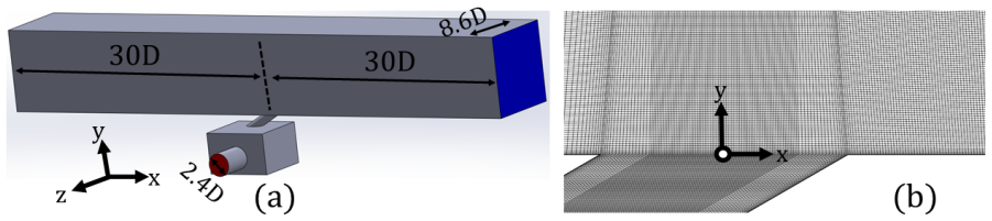
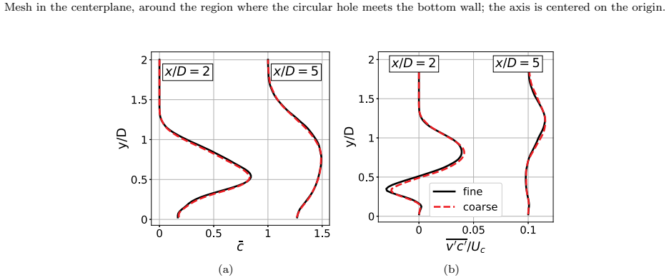
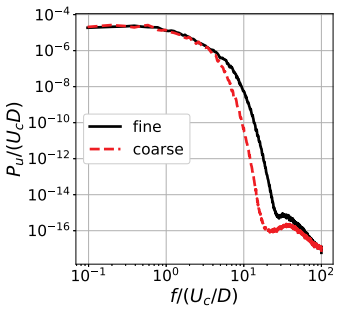
Summary. The paper presents a methodology to use highly resolved Large Eddy Simulations (LES) to complement and enrich three-dimensional mean flow measurements obtained by Magnetic Resonance Velocimetry (MRV) and Magnetic Resonance Concentration (MRC). The approach is demonstrated on a circular, 30-degree inclined jet in crossflow at velocity ratios r = 1, 1.5, and 2. The LES models the same geometry and flow conditions as the experiments, including the plenum and hole, and uses an iterative procedure to set inlet conditions that reproduce hot-wire profiles of the incoming boundary layer. The numerical meshes are highly refined (40-48 million cells), the subgrid-scale viscosity is small, and a coarse/fine mesh convergence study is performed. A validation campaign against the MRV/MRC mean fields is carried out using qualitative contour comparisons, one-dimensional profiles, and an integral circulation metric with misalignment-based error bars. After validation, the paper presents enrichment products that MRI cannot provide directly: wall concentration (adiabatic effectiveness), in-hole velocity, and turbulence statistics such as Reynolds stresses and turbulent scalar fluxes.
Significance. The proposed enrichment strategy is timely and potentially very useful: it exploits the full 3D volumetric validation that MRI uniquely offers, and then uses the validated LES to supply near-wall and second-moment data that MRI cannot measure. The paper demonstrates unusual care in matching experimental and numerical conditions: the iterative inlet-condition generation, long averaging times with a convergence check, mesh convergence study, and explicit propagation of misalignment uncertainty into the circulation comparison are all commendable and set a high standard for this type of hybrid experimental-numerical dataset. If the extrapolation to unmeasured quantities is accepted, the resulting datasets would be valuable for turbulence model development in film-cooling flows. The main risk is that this extrapolation rests entirely on agreement of mean fields; the paper should either strengthen that link or qualify the claims accordingly.
major comments (3)
- [Abstract and Sec. 5 (Conclusion); Sec. 4.3] The abstract and conclusion describe the LES as a 'validated set of simulations,' but the validation evidence is confined to mean velocity and mean scalar fields. The turbulence statistics in Sec. 4.3 (u'v' and v'c') and the near-wall concentration in Fig. 11 are enrichment products that are not checked against any independent measurement. The argument that agreement in resolvable mean 3D fields justifies trust in unmeasured fluctuation and near-wall quantities is plausible but not automatic; a simulation can match first moments while misrepresenting second moments. I recommend either adding a quantitative check of at least one turbulent correlation (e.g., using hot-wire or PIV in a representative plane) or explicitly labeling the turbulence and near-wall results as 'LES predictions not directly validated' and softening the wording in the abstract and conclusion.
- [Sec. 3.1, Eq. (5), and Fig. 11] The text states that setting the molecular Schmidt number to unity instead of the true value (of order 1000 for copper sulfate in water) has no practical effect because molecular diffusion is negligible compared to turbulent mixing, 'except extremely close to the bottom wall, where molecular diffusion might compete with turbulent mixing.' This caveat coincides exactly with the wall concentration (adiabatic effectiveness) presented as an enrichment result in Fig. 11, and the paper concedes 'there are no scalar data to be matched there.' Because the near-wall scalar value is sensitive to an unvalidated modeling choice, the authors should quantify the sensitivity (for example, by running the r = 1 case with Sc = 1000, or by a boundary-layer scaling argument) or else remove the wall concentration from the set of validated enrichment outputs.
- [Fig. 17(b)] The circulation comparison shows a consistent LES overprediction for all three velocity ratios, in several streamwise locations exceeding the 2-sigma misalignment error bars. This is the only quantitative integral metric used to validate the mean velocity field, so the systematic bias is a substantive discrepancy rather than minor scatter. The manuscript attributes it to 'other experimental uncertainties... or possible differences in the in-hole flow,' but no supporting evidence is provided. I ask the authors to investigate this bias (e.g., through a sensitivity study of the inlet-condition scaling factors or of the integration contour location) and to revise the phrase 'excellent agreement' in the conclusion so that it reflects this boundary of the validation.
minor comments (4)
- [Abstract] The word 'Velocimety' in the first sentence is a typo and should be 'Velocimetry.'
- [Sec. 2.1, Eq. (2)] The quantity SNR in Eq. (2) is not defined there; please define it explicitly as the signal-to-noise ratio measured as described in the text, ideally with the same symbol and definition used in the uncertainty estimate.
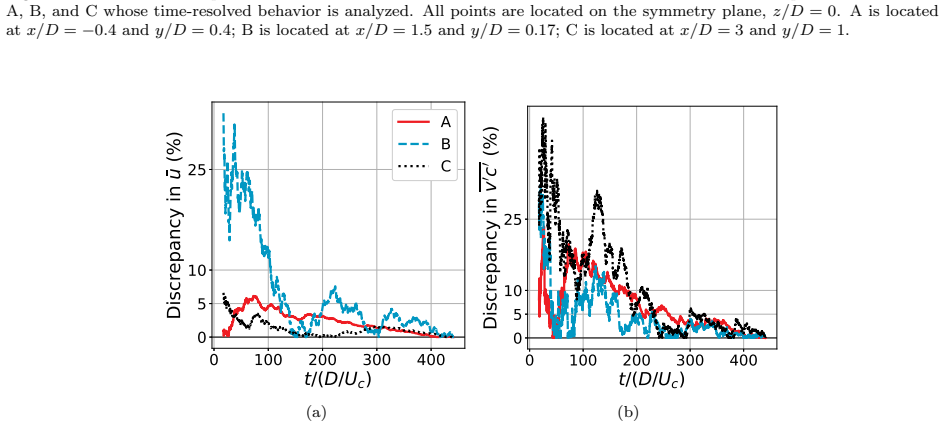
- [Fig. 8 caption] The phrase 'perceived time averages' is ambiguous; please replace it with 'running time averages' to clarify that the statistics accumulated up to each time step are compared with the final average.
- [Sec. 4.2, Fig. 17 caption] The text and figure legend use 'MRI data' while elsewhere the specific acronym 'MRV' is used; please be consistent throughout the manuscript.
Circularity Check
No circularity: LES validation and enrichment rely on independent MRV/MRC and hot-wire data, with no fitted quantity used as its own prediction.
full rationale
The derivation chain is self-contained against independent measurements. Inlet conditions are generated by an iterative channel-flow LES that is matched to hot-wire profiles of the same channel (Sec. 3.5, Table 2), and the hot-wire data are separate from the MRV/MRC datasets. The validation in Sec. 4 compares LES mean velocity and concentration fields directly with MRV and MRC experimental data acquired independently in Sec. 2. No prediction is defined in terms of the validated quantities: the near-wall scalar values, in-hole velocity details, and turbulent statistics (e.g., u'v' and v'c' in Sec. 4.3) are direct simulation outputs, not transformations of the MRI data. The SGS Schmidt number (0.85), molecular Schmidt number setting (Sc=1), and Vreman model are fixed modeling choices, not tuned to the experimental mean fields. The paper explicitly discloses that MRC data are unreliable very close to the wall and that the scalar field is insensitive to Sc except there, which is a limitation rather than a fitted-input/prediction loop. The circulation comparison (Fig. 17b) even shows a systematic LES overprediction, indicating the validation is not cherry-picked. Self-citations provide prior data and methods, but they are not load-bearing for the central validation claim. Concerns about extrapolating mean-field agreement to near-wall and turbulent statistics are legitimate correctness-risk concerns, not circularity of the derivation.
Assumptions & free parameters
free parameters (4)
- Inlet mean profile boundary-layer scale factor =
0.55
- Inlet u'rms amplification factor in boundary layer =
1.5
- Inlet u'rms amplification factor in freestream =
5
- Turbulent length scale for inlet generator =
0.7D
assumptions (4)
- domain assumption Filtered incompressible Navier-Stokes equations with Vreman SGS model govern the flow
- domain assumption Molecular Schmidt number Sc=1 adequately represents scalar mixing
- domain assumption Wall functions on side/top walls are acceptable
- domain assumption The hot-wire boundary layer data obtained in air at matched Reynolds number represent the water tunnel inlet
Cite this review
Pith. "Pith review of Enriching MRI mean flow data of inclined jets in crossflow with Large Eddy Simulations." pith.science (2026). https://pith.science/paper/CKGOISPW
@misc{pith2026190803540,
  author       = {Pith},
  title        = {Pith review of: Enriching MRI mean flow data of inclined jets in crossflow with Large Eddy Simulations},
  year         = {2026},
  howpublished = {\url{https://pith.science/paper/CKGOISPW}},
  note         = {Machine review of arXiv:1908.03540}
}
abstract
Measurement techniques such as Magnetic Resonance Velocimety (MRV) and Magnetic Resonance Concentration (MRC) are useful for obtaining 3D time-averaged flow quantities in complex turbulent flows, but cannot measure turbulent correlations or near-wall data. In this work, we use highly resolved Large Eddy Simulations (LES) to complement the experiments and bypass those limitations. Coupling LES and magnetic resonance experimental techniques is especially advantageous in complex non-homogeneous flows because the 3D data allow for extensive validation, creating confidence that the simulation results portray a physically realistic flow. As such we can treat the simulation as data, which "enrich" the original MRI mean flow results. This approach is demonstrated using a cylindrical and inclined jet in crossflow with three distinct velocity ratios, $r=1$, $r=1.5$, and $r=2$. The numerical mesh is highly refined in order for the subgrid scale models to have negligible contribution, and a systematic, iterative procedure is described to set inlet conditions. The validation of the mean flow data shows excellent agreement between simulation and experiments, which creates confidence that the LES data can be used to enrich the experiments with near-wall results and turbulent statistics. We also discuss some mean flow features and how they vary with velocity ratio, including wall concentration, the counter rotating vortex pair, and the in-hole velocity.
Figures


Figures from the paper (16 more)




Reference graph
Works this paper leans on
-
[1]
C. J. Elkins, M. Markl, N. Pelc, J. K. Eaton, 4D Magnetic Resonance Velocimetry for Mean Velocity Measurements in Complex Turbulent Flows, Experiments in Fluids 34 (2003) 494–503
work page 2003
-
[2]
M. J. Benson, C. J. Elkins, P. D. Mobley, M. T. Alley, J. K. Eaton, Three-dimensional Concentration Field Measurements in a Mixing Layer using Magnetic Resonance Imaging, Experiments in Fluids 49 (2010) 43–55
work page 2010
-
[3]
D. Freudenhammer, E. Baum, B. Peterson, B. B¨ ohm, B. Jung, S. Grundmann, Volumetric Intake Flow Measurements of an IC Engine Using Magnetic Resonance Velocimetry, Experiments in Fluids 55 (2014) 1724
work page 2014
-
[4]
N. W. Siegel, A. P. Schlenker, K. D. Sullivan, I. Valdez, G. P. Rodebaugh, C. J. Elkins, B. Van Poppel, M. J. Benson, Design and Analysis of a Spin Stabilized Projectile Using Magnetic Resonance Velocimetry, in: AIAA Scitech 2019 Forum, 2019, p. 0843. doi: 10.2514/6.2019-0843
-
[5]
G. Shim, D. Prasad, C. J. Elkins, J. K. Eaton, M. J. Benson, 3D MRI Measurements of the Effects of Wind Direction on Flow Characteristics and Contaminant Dispersion in a Model Urban Canopy, Environmental Fluid Mechanics (2019) 1–28
work page 2019
-
[6]
D. S. Ching, C. J. Elkins, J. K. Eaton, Investigation of Geometric Sensitivity of a non-Axisymmetric Bump: 3D Mean Velocity Measurements, Experiments in Fluids 59 (2018) 143
work page 2018
-
[7]
Mahesh, The Interaction of Jets With Crossflow, Annual Review of Fluid Mechanics 45 (2013) 379–407
K. Mahesh, The Interaction of Jets With Crossflow, Annual Review of Fluid Mechanics 45 (2013) 379–407. 21
work page 2013
-
[8]
D. G. Bogard, K. A. Thole, Gas Turbine Film Cooling, Journal of Propulsion and Power 22 (2006) 249–270
work page 2006
Show all 30 references
-
[9]
T. F. Fric, A. Roshko, Vortical Structure in the Wake of a Transverse Jet, Journal of Fluid Mechanics 279 (1994) 1–47
1994
-
[10]
L. K. Su, M. G. Mungal, Simultaneous Measurements of Scalar and Velocity Field Evolution in Turbulent Crossflowing Jets, Journal of Fluid Mechanics 513 (2004) 1–45
2004
-
[11]
Muppidi, K
S. Muppidi, K. Mahesh, Direct Numerical Simulation of Passive Scalar Transport in Transverse Jets, Journal of Fluid Mechanics 598 (2008) 335–360
2008
-
[12]
Kohli, D
A. Kohli, D. G. Bogard, Turbulent Transport in Film Cooling Flows, Journal of Heat Transfer 127 (2005) 513–520
2005
-
[13]
Schreivogel, C
P. Schreivogel, C. Abram, B. Fond, M. Straußwald, F. Beyrau, M. Pfitzner, Simultaneous kHz-rate Temperature and Velocity Field Measurements in the Flow Emanating from Angled and Trenched Film Cooling Holes, International Journal of Heat and Mass Transfer 103 (2016) 390–400
2016
-
[14]
Coletti, M
F. Coletti, M. J. Benson, J. Ling, C. J. Elkins, J. K. Eaton, Turbulent Transport in an Inclined Jet in Crossflow, International Journal of Heat and Fluid Flow 43 (2013) 149–160
2013
-
[15]
K. J. Ryan, Three-Dimensional Velocity and Concentration Measurements of Turbulent Mixing in Discrete Hole Film Cooling, PhD Thesis, Stanford University, Stanford, CA, 2016. URL: http://purl.stanford.edu/vy115tc2952
2016
-
[16]
Schiavazzi, F
D. Schiavazzi, F. Coletti, G. Iaccarino, J. K. Eaton, A Matching Pursuit Approach to Solenoidal Filtering of three- Dimensional Velocity Measurements, Journal of Computational Physics 263 (2014) 206–221
2014
-
[17]
N. J. Pelc, F. G. Sommer, K. C. Li, T. J. Brosnan, R. J. Herfkens, D. R. Enzmann, Quantitative Magnetic Resonance Flow Imaging, Magnetic Resonance Quarterly 10 (1994) 125–147
1994
-
[18]
C. J. Elkins, M. T. Alley, Magnetic Resonance Velocimetry: Applications of Magnetic Resonance Imaging in the Mea- surement of Fluid Motion, Experiments in Fluids 43 (2007) 823–858
2007
-
[19]
S. D. Yapa, J. L. DAtri, J. M. Schoech, C. J. Elkins, J. K. Eaton, Comparison of Magnetic Resonance Concentration Measurements in Water to Temperature Measurements in Compressible Air Flows, Experiments in Fluids 55 (2014) 1834
2014
-
[20]
Hultmark, A
M. Hultmark, A. Smits, Temperature Corrections for Constant Temperature and Constant Current Hot-wire Anemometers, Measurement Science and Technology 21 (2010) 105404
2010
-
[21]
Emanuel, D
A. Emanuel, D. R. Olander, Diffusion Coefficients of Copper Sulfate in Water and Water in n-Butyl Alcohol, Journal of Chemical and Engineering Data 8 (1963) 31–32
1963
-
[22]
A. W. Vreman, An Eddy-Viscosity Subgrid-Scale Model for Turbulent Shear Flow: Algebraic Theory and Applications, Physics of Fluids 16 (2004) 3670–3681
2004
-
[23]
F. Ham, An Efficient Scheme for Large Eddy Simulation of Low-Ma Combustion in Complex Configurations, Annual Research Briefs, Center for Turbulence Research, Stanford University, Stanford, CA (2007) 41–46
2007
-
[24]
D. K. Walters, J. H. Leylek, A Systematic Computational Methodology Applied to a Three-Dimensional Film-Cooling Flowfield, Journal of Turbomachinery 119 (1997) 777–785
1997
-
[25]
Muppidi, K
S. Muppidi, K. Mahesh, Direct Numerical Simulation of Round Turbulent Jets in Crossflow, Journal of Fluid Mechanics 574 (2007) 59–84
2007
-
[26]
Bodart, F
J. Bodart, F. Coletti, I. Bermejo-Moreno, J. K. Eaton, High-Fidelity Simulation of a Turbulent Inclined Jet in a Crossflow, Center for Turbulence Research Annual Research Briefs (2013) 263–275
2013
-
[27]
Cabot, P
W. Cabot, P. Moin, Approximate Wall Boundary Conditions in the Large-Eddy Simulation of High Reynolds Number Flow, Flow, Turbulence and Combustion 63 (2000) 269–291
2000
-
[28]
Z. T. Xie, I. P. Castro, Efficient Generation of Inflow Conditions for Large Eddy Simulation of Street-Scale Flows, Flow, Turbulence and Combustion 81 (2008) 449–470
2008
-
[29]
P. M. Milani, J. Ling, G. Saez-Mischlich, J. Bodart, J. K. Eaton, A Machine Learning Approach for Determining the Turbulent Diffusivity in Film Cooling Flows, Journal of Turbomachinery 140 (2018) 021006
2018
-
[30]
S. H. Smith, M. G. Mungal, Mixing, Structure and Scaling of the Jet in Crossflow, Journal of Fluid Mechanics 357 (1998) 83–122. 22
1998
Reviewed August 14, 2026 · model on record in the stance chip above.
Discussion (0). Continue with ORCID to comment.