REVIEW 4 major objections 5 minor 32 references
Quasi-spectral characterization of intracellular regions in bright-field light microscopy images
T0 review · 4 major / 5 minor · reviewed 2026-08-14 · deepseek-v4-flash
Pith's one-line read The paper argues that per-pixel transparency-like spectra, recovered from ordinary bright-field images via a regularized inverse problem, carry enough physical information to segment unstained cells better than raw RGB.
desk verdict A genuinely useful feature-extraction pipeline for bright-field microscopy, but the 'physically correct spectra' claim is unsupported and the main validation is circular. read the letter →
The pith
A machine-rendered reading of the paper's core claim, the machinery that carries it, and where it could break.
The reading
What carries the argument
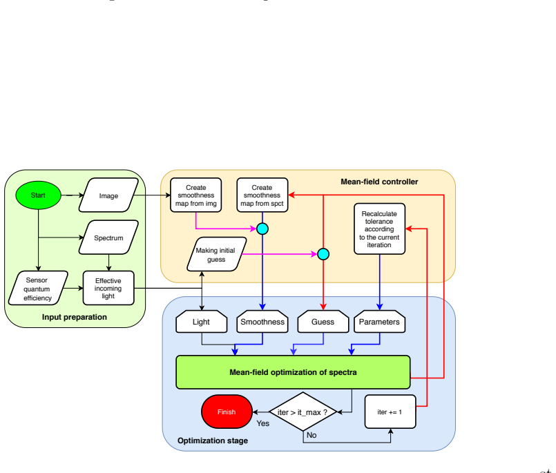
The central object is the per-pixel quasi-spectrum $T_m(\lambda)$, discretized into 48 wavelengths, recovered by minimizing the per-pixel cost $F_m$ in Eq. 4. The first term enforces consistency with the measured channel intensities $I_m$ under the effective incoming light $L_c(\lambda)=S(\lambda)F_c(\lambda)$; the second term enforces spectral smoothness across neighbouring pixels, with the smoothness weight $G_{mn}$ (Eq. 5) reduced at edge pixels via Canny edge detection and at steep gradient locations. The machinery is the mean-field iterative optimization: each pixel's spectrum is optimized while neighbour spectra are fixed, the smoothness map is recomputed from the current spectral guess by zero-lag cross-correlation, and a robust global optimization method (CMA-ES) is used for the local minimization.
What would settle it
Record a sample whose transmission spectrum can be measured independently (for example, a thin uniform filter over a range of wavelengths) on the same microscope, run the quasi-spectral reconstruction, and compare the recovered $T_m(\lambda)$ to the spectrophotometer measurement at each wavelength; if the curves deviate systematically beyond the calibration error, the recovered spectra are not transparency spectra, although they might still be useful features.
Extended reading notes
Core claim
The paper's central claim is that solving the regularized inverse problem of Eq. 4 recovers, for each pixel, a 48-point curve $T_m(\lambda)$ that behaves as a transparency spectrum. The optimization balances reproduction of the three measured channel intensities against a smoothness penalty over neighbouring pixels, with the penalty weight $G_{mn}$ reduced where edge detection and intensity gradients indicate object boundaries. Because the recovered curves reproduce the original image under re-illumination and cluster into classes that are stable across different cells, the authors take them to be physically relevant features, while explicitly conceding that the identity with true transparency is not proven due to a lack of reference data. The rest of the paper documents unsupervised clustering and supervised segmentation results that support the method's practical value.
Load-bearing premise
The load-bearing premise is that requiring neighbouring pixels to have similar spectra, with discontinuities only at detected edges, is enough to turn three intensity measurements per pixel into one unique, physically meaningful 48-point spectrum.
Editorial extensions
If this is right
- Unstained living cells can be segmented into regions with distinct quasi-spectra without any training data, purely by unsupervised clustering of the recovered curves.
- Supplying quasi-spectra instead of raw RGB to a supervised segmentation network raises Intersection over Union by more than 10% and reaches maximum performance in about 8 epochs instead of 40.
- Because the recovered spectra are illumination-independent in the model, images can be re-rendered under arbitrary illumination (for example, a black-body spectrum at 5800 K) and still match the original scene.
- The same extraction pipeline applies to any bright-field microscope with a linear camera response, as long as the incoming light spectrum and camera filter profiles are measured or supplied.
Reading between the lines
- A natural falsification test the authors do not report: record the same field of view with a spectrophotometer or a tunable light source, and compare the recovered quasi-spectra to measured transmission spectra; agreement would separate the smoothness prior's regularizing role from a genuine spectral estimate.
- The recovered curves likely conflate thickness with composition: since transmission multiplies along the optical path, a thicker pixel of the same material would integrate lower transmission, an effect the cosine-distance clustering deliberately discards.
- The same inverse formulation could be adapted to other 3-channel imaging systems, including endoscopy or satellite imagery, wherever effective illumination and sensor response curves are known; the paper's own claims are limited to microscopy, but the structure of Eq. 2 is not.
Signed reviews
Editorial analysis
A structured set of objections, weighed in public.
Referee Report
Summary. The paper introduces an algorithm that, from a standard RGB bright-field microscopy image, estimates a per-pixel 'quasi-transparency spectrum' T_m(λ) by solving a regularized inverse problem. The forward model (Eq. 2) assumes a linear response: each color channel is an integral of the product of the incoming light spectral profile L_c(λ) and the unknown transparency spectrum. Because the problem is underdetermined, the authors add a spatial smoothness prior (Eq. 3) with an edge-aware weighting G_mn (Eq. 5), and optimize the resulting cost (Eq. 4) iteratively with CMA-ES. The paper reports three forms of evaluation: artificial re-illumination of the recovered spectra (Fig. 4c), gap-statistics comparison of k-means clustering on spectra versus raw RGB (Fig. 5g), and U-Net semantic segmentation (Fig. 4f), plus phantom experiments on oil-air and egg-protein-air interfaces. The authors state explicitly that they lack reference data to prove that the recovered feature vectors coincide with true transparency spectra, and they describe their outputs as 'quasi-spectra' throughout most of the text.
Significance. If the central claim were supported, the method would be a practical, low-cost way to attach spectral-like information to ordinary bright-field images, with potential applications in label-free cell biology. The paper has genuine strengths: it ships reproducible code and data, performs careful per-pixel camera calibration, uses large pixel-statistics gap analysis, includes phantom and deep-learning segmentation comparisons, and is unusually candid about its limitations, including the absence of ground-truth spectra. However, the central physical-correctness claim is currently not established: no identifiability analysis is given for the heavily underdetermined inverse problem, the main 're-illumination' validation is circular, and the paper contains no test against measured transmission spectra. The empirical clustering and segmentation improvements appear real, but they support the usefulness of the transform as a feature extractor, not the physical interpretation of the recovered spectra.
major comments (4)
- [Optimization procedure, Eq. 4] The inverse problem is underdetermined: each pixel gives only C=3 intensity constraints (RGB) while the discrete spectrum has w=48 unknowns. The spatial smoothness term (Eq. 3) couples neighboring pixels but does not, by itself, select a unique or physically meaningful spectrum; any sufficiently smooth function in the nullspace of the three projection kernels L_c(λ) can be added to a particular solution without changing the data term. The paper provides no identifiability analysis, no test with known ground-truth spectra, and no sensitivity analysis demonstrating that the recovered spectra are determined by the data rather than by the choice of regularization. This is load-bearing because the abstract and Introduction claim 'physically correct extraction' of features resembling transparency spectra. The authors should either provide such an analysis (for example, synthetic phantoms with known spectra) or reframe the contribution as a nonlinear feature transform whose physical interpretation is not claimed.
- [Results, Fig. 4c and surrounding text] The artificial re-illumination check is circular as a validation of physical correctness. The reconstructed spectra are obtained by minimizing the discrepancy between the model integrals (Eq. 2) and the RGB image; re-integrating the same spectra with the same L_c(λ) and displaying the result will necessarily resemble the input image, even if the spectra are arbitrary smooth functions consistent with the three per-pixel integrals. This is not an independent prediction. To support the physical interpretation, the authors need a validation against measured transmission spectra of known samples (e.g., using the same spectrophotometer setup as in their calibration), or a cross-validation scheme in which a subset of spectral channels is withheld during fitting and predicted from the remainder.
- [Discussion, 'It is worth mentioning...'] The transparency coefficient is physically bounded by [0,1], and the Discussion states this bound, but the optimization target in Eq. 4 as written does not enforce T_m(λ)∈[0,1]. The paper later excludes 'light-condensing' objects whose spectra violate the model, but it does not report what fraction of pixels are affected, nor whether the remaining spectra lie in the physically admissible range. Without either an explicit constraint in the optimization or a post-hoc check that the recovered spectra respect the bound, the claim that the features are 'physically correct' is unsupported even in regions where the measurement model is assumed to hold.
- [Evaluation of the asset, Fig. 5g and phantom experiments] The clustering and phantom results show that the quasi-spectral transform improves cluster separation relative to raw RGB, but they do not discriminate among alternative spectral reconstructions: a different regularization that produced different spectra but equally good separation would pass the same tests. The paper states that the method is 'quite robust to parametrization inaccuracies' but provides no systematic study of the many free parameters (T_b, TED, w, Gaussian sigma, edge-detection settings, number of clusters k). A robustness study, or at least a scan over the main hyperparameters, is needed to establish that the reported improvements are not artifacts of a particular parameter choice.
minor comments (5)
- [Equation 4] The first term in Eq. 4 is typeset ambiguously: it reads 'e |∫... |' with no visible exponent, and the '-C + 1' after the sum is unclear. Please rewrite with explicit superscripts and parentheses so the intended exponential/absolute-value structure is unambiguous.
- [List of symbols and Eq. 5] The symbol T is used for both the transparency spectrum T(λ) and thermodynamic temperature T in the List of Symbols, and the bias parameter appears as both T_b in Eq. 5 and Tb in the text; please disambiguate.
- [Throughout] The text frequently uses 'Authors used' (e.g., 'Authors used TED = 1', 'Authors used the Simpson integration method') in a paper whose authors are the same people; this should be changed to first-person ('we used') or passive voice.
- [Figure 4 caption] In the caption to Fig. 4, 'absolute black body' should be 'ideal black body' or 'Planckian radiator'; also 'arbitrary illumination such as the absolute black body' could be clearer.
- [Abstract and Introduction] The abstract and Introduction use the phrase 'physically correct extraction', while the body repeatedly and correctly emphasizes that only 'quasi-spectra' are obtained and that strict proof is absent. The strong phrase should be softened in the abstract to match the actual scope of the claims.
Circularity Check
No significant circularity: the regularized inverse problem is not equivalent to its inputs, and the re-illumination check uses a different illuminant and CIE color-matching functions, not the same camera model.
full rationale
The derivation chain is: Eq. 2 gives the RGB forward model; Eq. 4 defines a regularized inverse problem with a data-fidelity term plus a spatial L2-smoothness prior weighted by G_mn (Eq. 5). This is not a self-definitional reduction: the optimizer is underdetermined (3 constraints vs 48 unknowns), but the smoothness prior and edge weighting are additional assumptions, not a restatement of the measured intensities. The paper's main validity check, artificial re-illumination (Fig. 4c), is described as multiplying the recovered spectra by a 5800 K black-body spectrum and CIE 1931 standard matching curves; this is not the same forward model as Eq. 2, which uses the measured effective incoming light L_c. The resemblance is therefore not forced by construction. It is a weak consistency check, not a circular prediction. The calibration procedure uses independent gray-filter images and a spectrophotometer, and the clustering/segmentation tests (gap statistics, phantom oil/air and egg-protein interfaces, U-Net) are external comparisons that do not presuppose the recovered spectra. The paper explicitly concedes 'the lack of reference data (to prove strictly that the proposed feature vectors coincide with transparency)' and states 'some information is irrecoverably lost'; underdetermination and identifiability are correctness and validation limitations, not circularity. The only self-citations (Ref. 1 on the microscope setup and effective-focus position; Ref. 30 for deposited code/data) are not load-bearing for the central derivation and are not invoked as a uniqueness theorem. No Eq. X = Eq. Y reduction or fitted-parameter-renamed-as-prediction step is exhibited.
Assumptions & free parameters
free parameters (5)
- T_b (bias parameter) =
0.9
- TED (neighborhood radius) =
1 pixel
- w (discrete wavelength count) =
48
- Gaussian sigma for edge smoothing =
0.5
- k (number of clusters) =
10
assumptions (6)
- domain assumption Linearity of the imaging model (Eq. 2): I_c = integral of L_c(lambda) T(lambda) d lambda, with no scattering, fluorescence, or optics effects.
- domain assumption Source spectrum S(lambda) is constant, known, and spatially homogeneous during acquisition.
- domain assumption Camera quantum efficiency curves Fc(lambda) from the vendor are accurate.
- ad hoc to paper Spatial continuity (Eq. 3): neighboring pixels have similar transparency spectra except at edges.
- ad hoc to paper The smoothness weighting G_mn (Eq. 5) correctly identifies discontinuities and does not bias spectra.
- domain assumption Sample thickness and focus do not change spectral shape, only integral magnitude.
invented entities (1)
-
Per-pixel quasi-transparency spectrum T_m(lambda)
Cite this review
Pith. "Pith review of Quasi-spectral characterization of intracellular regions in bright-field light microscopy images." pith.science (2026). https://pith.science/paper/EEDI33KE
@misc{pith2026190803696,
  author       = {Pith},
  title        = {Pith review of: Quasi-spectral characterization of intracellular regions in bright-field light microscopy images},
  year         = {2026},
  howpublished = {\url{https://pith.science/paper/EEDI33KE}},
  note         = {Machine review of arXiv:1908.03696}
}
read the original abstract
Investigation of cell structure is hardly imaginable without bright-field microscopy. Numerous modifications such as depth-wise scanning or videoenhancement make this method being state-of-the-art. This raises a question what maximal information can be extracted from ordinary (but well acquired) bright-field images in a model-free way. Here we introduce a method of a physically correct extraction of features for each pixel when these features resemble a transparency spectrum. The method is compatible with existent ordinary bright-field microscopes and requires mathematically sophisticated data processing. Unsupervised clustering of the spectra yields reasonable semantic segmentation of unstained living cells without any a priori information about their structures. Despite the lack of reference data (to prove strictly that the proposed feature vectors coincide with transparency), we believe that this method is the right approach to an intracellular (semi)quantitative and qualitative chemical analysis.
Figures


Figures from the paper (2 more)


Reference graph
Works this paper leans on
-
[1]
Rychtáriková, R.et al. Super-resolved 3-d imaging of live cells organelles’ from bright- field photon transmission micrographs.Ultramicroscopy179, 1–14 (2017)
work page 2017
-
[2]
Lindner, M., Shotan, Z. & Garini, Y. Rapid microscopy measurement of very large spectral images. Optics Express24, 9511 (2016)
work page 2016
-
[3]
Heist, S. et al. 5D hyperspectral imaging: fast and accurate measurement of surface shape and spectral characteristics using structured light. Optics Express 26, 23366 (2018)
work page 2018
-
[4]
Wu, J.et al.Snapshot hyperspectral volumetric microscopy.Scientific Reports6, 24624 (2016)
work page 2016
-
[5]
Wachman, E. S. et al. Simultaneous imaging of cellular morphology and multiple biomarkers using an acousto-optic tunable filter–based bright field microscope.Jour- nal of Biomedical Optics19, 056006 (2014)
work page 2014
-
[6]
Dahlberg, P. D.et al. A simple approach to spectrally resolved fluorescence and bright field microscopy over select regions of interest.Review of Scientific Instruments87, 113704 (2016)
work page 2016
- [7]
-
[8]
Garini, Y., Young, I. T. & McNamara, G. Spectral imaging: Principles and applications. Cytometry Part A69A, 735–747 (2006)
work page 2006
Show all 32 references
-
[9]
Maloney, L. T. Evaluation of linear models of surface spectral reflectance with small numbers of parameters.Journal of the Optical Society of America A3, 1673 (1986)
1986
-
[10]
& Wandell, B
Parmar, M., Lansel, S. & Wandell, B. A. Spatio-spectral reconstruction of the multi- spectral datacube using sparse recovery. In2008 15th IEEE International Conference on Image Processing(IEEE, 2008)
2008
-
[11]
& Huang, B
Wang, Y., Yang, B., Feng, S., Pessino, V. & Huang, B. Multicolor fluorescent imaging by space-constrained computational spectral imaging.Optics Express27, 5393 (2019)
2019
-
[12]
& Garrote, E
Alvarez-Gila, A., van de Weijer, J. & Garrote, E. Adversarial networks for spatial context-aware spectral image reconstruction from RGB. In 2017 IEEE International Conference on Computer Vision Workshops (ICCVW)(IEEE, 2017)
2017
-
[13]
Hoover, E. E. & Squier, J. A. Advances in multiphoton microscopy technology.Nature Photonics 7, 93–101 (2013)
2013
-
[14]
Lugagne, J.-B. et al. Identification of individual cells from z-stacks of bright-field mi- croscopy images.Scientific Reports8, 11455 (2018). 12
2018
-
[15]
Velleman, D. J. The generalized Simpson’s rule.The American Mathematical Monthly 112, 342 (2005)
2005
-
[16]
Kuzmin, Y. P. Bresenham’s line generation algorithm with built-in clipping.Computer Graphics Forum14, 275–280 (1995)
1995
-
[17]
A computational approach to edge detection.IEEE Transactions on Pattern Analysis and Machine IntelligencePAMI-8, 679–698 (1986)
Canny, J. A computational approach to edge detection.IEEE Transactions on Pattern Analysis and Machine IntelligencePAMI-8, 679–698 (1986)
1986
-
[18]
& Werman, M
Elboher, E. & Werman, M. Efficient and accurate Gaussian image filtering using run- ning sums. In 2012 12th International Conference on Intelligent Systems Design and Applications (ISDA)(IEEE, 2012)
2012
-
[19]
On lines and planes of closest fit to systems of points in space.The London, Edinburgh, and Dublin Philosophical Magazine and Journal of Science2, 559–572(1901)
Pearson, K. On lines and planes of closest fit to systems of points in space.The London, Edinburgh, and Dublin Philosophical Magazine and Journal of Science2, 559–572(1901)
1901
-
[20]
& Anderson, R
Hair, J., Black, W., Babin, B. & Anderson, R. Multivariate Data Analysis (Cen- gage Learning EMEA, 2018). URL https://www.ebook.de/de/product/33402106/ university_of_south_alabama_joseph_hair_william_black_barry_louisiana_ tech_university_babin_rolph_drexel_university_anderson...
2018
-
[21]
& Ostermeier, A
Hansen, N. & Ostermeier, A. Completely derandomized self-adaptation in evolution strategies. Evolutionary Computation9, 159–195 (2001)
2001
-
[22]
The CMA evolution strategy: A comparing review
Hansen, N. The CMA evolution strategy: A comparing review. In Lozano, J., Larranaga, P., Inza, I. & Bengoetxea, E. (eds.)Towards a New Evolutionary Computation, 75–102 (Springer Berlin Heidelberg, 2007)
2007
-
[23]
& Fernandez-Valdivia, J
Pech-Pacheco, J., Cristobal, G., Chamorro-Martinez, J. & Fernandez-Valdivia, J. Di- atom autofocusing in brightfield microscopy: a comparative study. InProceedings 15th International Conference on Pattern Recognition. ICPR-2000 (IEEE Comput. Soc., 2002)
2000
-
[24]
& Wongsa, S
Mekaroonkamon, T. & Wongsa, S. A comparative investigation of the robustness of unsupervised clustering techniques for rotating machine fault diagnosis with poorly- separated data. In 2016 Eighth International Conference on Advanced Computational Intelligence (ICACI)(IEEE, 2016)
2016
-
[25]
& Hastie, T
Tibshirani, R., Walther, G. & Hastie, T. Estimating the number of clusters in a data set via the gap statistic.Journal of the Royal Statistical Society: Series B (Statistical Methodology)63, 411–423 (2001)
2001
-
[26]
Technique of factor analysis.Nature 136, 297 (1935)
Stephenson, W. Technique of factor analysis.Nature 136, 297 (1935)
1935
-
[27]
Lee, D. D. & Seung, H. S. Learning the parts of objects by non-negative matrix factor- ization. Nature 401, 788–791 (1999). 13
1999
-
[28]
& Brox, T
Ronneberger, O., Fischer, P. & Brox, T. U-net: Convolutional networks for biomedical image segmentation. In Navab, N., Hornegger, J., Wells, W. M. & Frangi, A. F. (eds.) Medical Image Computing and Computer-Assisted Intervention – MICCAI 2015, 234– 241 (Springer International ...
2015
-
[29]
Lichtscheidl, I. K. & Foissner, I. Video microscopy of dynamic plant cell organelles: principles of the technique and practical application.Journal of Microscopy181, 117– 128 (1998)
1998
-
[30]
& ’tys, D
Lonhus, K., Rychtáriková, R., Platonova, G. & ’tys, D. Supplementary toQuasi-spectral characterization of intracellular regions in bright-field light microscopy images. Dryad, Dataset URL https://doi.org/10.5061/dryad.w0vt4b8p6. ACKNOWLEDGEMENTS This work was supported by the M...
-
[31]
Experimental Part: a. Using a microscope photocamera, images (raw files) of the set of gray layers covering a 2 mm thick glass (type Step ND Filter NDL–10S–4) on a microscope stage were captured successively. The image of zero and the highest intensity was acquired at zero phot...
-
[32]
Construction of a calibration curve for each pixel (1) Red, green, and blue camera Bayer filter profiles (supplied by a camera producer; Fig
Computational Part: a. Construction of a calibration curve for each pixel (1) Red, green, and blue camera Bayer filter profiles (supplied by a camera producer; Fig. 3b) were transformed into the numeric format. The results are saved in the spectrum.txt file of the calibration dat...
2001
Reviewed August 14, 2026 · model on record in the stance chip above.
Discussion (0). Continue with ORCID to comment.