REVIEW 4 major objections 4 minor 25 references
Coexistence of hidden attractors and self-excited attractors through breaking heteroclinic-like orbits of switched systems
T0 review · 4 major / 4 minor · reviewed 2026-08-14 · deepseek-v4-flash
Pith's one-line read This paper claims that a hidden attractor emerges in a piecewise linear switched system when the switching plane between two self-excited double-scroll attractors is moved so that trajectories that would be funneled into those attractors…
desk verdict Genuine construction paper with a plausible hidden-attractor mechanism, but the trapping-region proof has a numerical gap and rests on an assumption not validated in 3D. read the letter →
The pith
A machine-rendered reading of the paper's core claim, the machinery that carries it, and where it could break.
The reading
What carries the argument
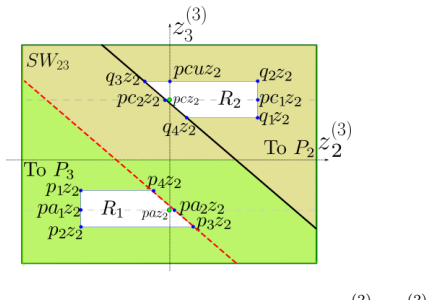
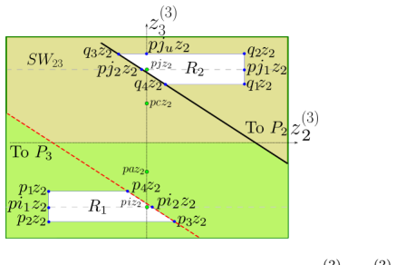
The load-bearing object is the switching surface $SW_{23}$, moved from the plane $2x_1-x_3=0$ to the plane $x_1=0$ while the other two switching surfaces stay in place. On this surface the authors define two trapping regions $R_1$ and $R_2$ by four corner points each, chosen so that the funneling subsets $I_1$ and $I_2$ (the neighborhoods of the heteroclinic connection points $p_a$ and $p_c$) no longer intersect them. The proof that trajectories in $R_1$ reach $R_2$ or a self-excited attractor rests on comparing radii of rotation in the $z^{(2)}$ coordinate system, using the explicit linear diagonalization $A=QEQ^{-1}$ with eigenvalues $c$, $a\pm ib$, and on the approximation that a 270-degree rotation in the full three-dimensional system grows in radius about as much as a rotation around a single equilibrium in the two-dimensional projection.
What would settle it
Integrate the full system (1), (2), (4), (23) and (107) with $a=0.2$, $b=5$, $c=-7$, $\alpha=1$, $\gamma=10$ from $x_0=(0,0,0)$ for time well beyond the reported window; if the trajectory eventually converges to one of the two self-excited double-scroll attractors rather than continuing to cross $R_1$ and $R_2$, then the claimed hidden attractor is not an attractor. A second check: compare the radius growth over a 270-degree arc in the full system with the prediction of the reduced system (77); a mismatch larger than the inequalities allow would break the trapping proof.
Extended reading notes
Core claim
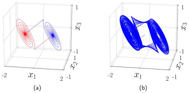
The central claim is that the system defined by (1), (2), (4), (23) and (107) with $a=0.2$, $b=5$, $c=-7$, $\alpha=1$ and $\gamma=10$ possesses a hidden attractor that coexists with two self-excited double-scroll attractors. The hidden attractor arises because the modified switching surface $SW_{23}=\{x\in\mathbb{R}^3: x_1=0\}$ makes the regions $R_1$ and $R_2$ on that surface disjoint from the subsets $I_1$ and $I_2$ that would otherwise funnel trajectories into the self-excited attractors. The paper verifies this by constructing trapping regions on $SW_{23}$, proving that trajectories starting in $R_1$ reach $R_2$ or a self-excited attractor and vice versa, and showing numerically that for $\gamma=10$ the claimed hidden attractor persists over long time windows.
Load-bearing premise
The trapping-region construction rests on the approximation that a 270-degree rotation in the full three-dimensional system grows in radius about the same as a rotation around a single equilibrium in a two-dimensional projection, checked only on a reduced two-dimensional system with a hysteresis function, together with the parameter regime $b/a\ge 25$, $2\ge |c/b|\ge 7/5$, $\gamma/\alpha\ge 10$.
Editorial extensions
If this is right
- For the parameter set $a=0.2$, $b=5$, $c=-7$, $\alpha=1$, $\gamma=10$, the system has a hidden attractor plus two self-excited double-scroll attractors, so multistability occurs without any equilibria inside the hidden attractor's basin.
- Moving only the middle switching surface to $x_1=0$ preserves the two heteroclinic loops and therefore preserves the two self-excited attractors while enabling the hidden one.
- For sufficiently large $\gamma$, the intersections $N(p_a)\cap R_1$ and $N(p_c)\cap R_2$ are empty, so no trajectory is forced into a self-excited attractor; the paper's inequalities give explicit parameter conditions of this kind.
- Trajectories starting in $R_1$ must reach $R_2$ or a self-excited attractor, and symmetrically for $R_2$, so any hidden attractor must pass through both regions.
- The construction indicates a geometric route to multistable PWL systems with coexistence of hidden and self-excited attractors, and possibly to systems with no equilibria at all.
Reading between the lines
- A testable extension is to scan $\gamma$ continuously in the same four-equilibrium system: the paper's inequalities predict that the hidden attractor should appear only above a threshold where the funneling intersections vanish, and disappear again if $\gamma$ becomes so large that the rotational-radius approximation degrades.
- A direct numerical check of radius growth in the full three-dimensional system versus the reduced two-dimensional system (77) would settle whether Assumption 4 holds beyond the tested parameter range; if it fails, $R_1$ may leak trajectories into the self-excited basins.
- The same 'break the heteroclinic-like orbit' idea could be applied to chains of more than four equilibria, potentially producing several hidden attractors arranged between multiple self-excited attractors.
- Because the hidden attractor's basin of attraction contains no equilibria, the geometric construction may be adaptable to systems without equilibria, which the paper notes as a feasible direction.
Signed reviews
Editorial analysis
A structured set of objections, weighed in public.
Referee Report
Summary. The paper proposes a constructive approach for generating hidden attractors in piecewise-linear switched systems. Starting from a two-atom system with heteroclinic chaos (Section 2), the authors add two more equilibria (Section 3) to obtain two self-excited double-scroll attractors, and then modify the switching surface SW23 to x1=0 (Section 5) with the aim of blocking the routes to the self-excited attractors and thereby creating a hidden attractor. The main claim is that the system given by (1), (2), (4), (23), and (107) with a=0.2, b=5, c=-7, alpha=1, gamma=10 possesses a hidden attractor coexisting with two self-excited double-scroll attractors. The argument is a mix of analytic estimates for trapping regions R1 and R2, a set of parameter assumptions, and numerical simulations, with the final confirmation resting on the sentence 'Simulation experiments verify the conjecture on the emergence of the hidden attractor.'
Significance. If the central claim were rigorously established, the paper would offer a useful geometric design principle for multistable PWL systems with coexisting hidden and self-excited attractors, and it would connect hidden attractors to the breaking of large-scale heteroclinic-like orbits. The paper has notable strengths: an explicit and simple PWL construction, exact linear-flow formulas in Eq. (21), explicit parameter ranges in Assumptions 2 and 3, and numerical illustrations for several parameter regimes. However, the analytic trapping proof has a numerical gap at the final comparison, and the key Assumption 4 is validated only on a reduced planar model rather than on the original 3D system. These issues leave the principal hidden-attractor claim supported mainly by simulation, so the paper is currently more a numerical demonstration with a heuristic framework than a fully established result.
major comments (4)
- [Section 5, Eqs. (143)-(148)] The trapping verification for the region R1 does not deliver the claimed conclusion. The escape-radius bound is estimated as 1.1091*gamma in Eq. (145), while the minimum radius of the segment pa1z2-pa2z2 is bounded below by 1.1081*gamma in Eq. (148). The paper then writes '1.1092*gamma approximately 1.1081*gamma', but the required conclusion is 1.1091*gamma < 1.1081*gamma, and the printed numerical bounds go in the opposite direction. Since this comparison is exactly what is supposed to show that trajectories starting in R1 cannot reach the subsets I1/I2 and hence cannot be routed to the self-excited attractors, the gap is load-bearing for the hidden-attractor claim.
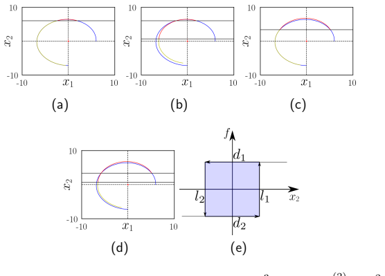
- [Section 4, Assumption 4, p. 24] Assumption 4 states that the increment in radius for a 270-degree rotation in the full 3D system is approximately the same as for a rotation around a single equilibrium in the 2D projection, but it is validated only on the reduced planar hysteresis system (77), not on the original system (1), (2), (4), (23), (107). All subsequent inequalities defining the trapping region R1 and the absence of escape routes depend on this approximation. If the true 3D radial growth is larger, trajectories from R2 could reach I2 and fall into a self-excited attractor. The paper should either prove a rigorous bound for the full 3D flow or provide direct 3D numerical verification for the parameter set used in Section 5.
- [Section 3, Proposition 3.1, p. 13-14] The derivation of the gamma interval Gamma mixes t<0 and t>0 analyses in a way that needs clarification. For the point pa on the heteroclinic orbit joining x_eq2 and x_eq3, the requirement is that the trajectory remains in P2 for all t<0, but the maximum of z_3^{(2)}(t) is then computed for t>0 using Eqs. (40)-(42). The same issue applies to the computation for pb. Since the interval (gamma_L, gamma_U) is used to assert the existence of six heteroclinic orbits and to distinguish the regimes in Figures 3 and 4, this inconsistency should be resolved before the heteroclinic-orbit count is relied upon.
- [Section 5, Fig. 13b] The evidence for the hidden attractor is a single trajectory segment for t in [50000, 50100] with initial condition x0=(0,0,0). Given the long transients documented earlier in the paper (about 350 a.u. for gamma=100 and about 3090 a.u. for gamma=1000), this one segment does not by itself rule out eventual convergence to one of the self-excited attractors. A direct longer-time integration, a basin-of-attraction computation, or an explicit invariant region in the full 3D system is needed to substantiate the claim that the attractor is genuinely hidden and persistent.
minor comments (4)
- [Abstract] There are several typographical errors: 'seft-excited' should be 'self-excited', 'biestability' should be 'bistability', and 'two self-excited attractor' should be 'two self-excited attractors'. The abstract also states that the approach 'consists of the coexistence' of attractors, which should be rephrased for clarity.
- [Eq. (107)] In Eq. (107) the switching surfaces are written with the union symbol, e.g., 'SW12 = cl(P1) union cl(P2)', whereas the earlier definition in Section 2 correctly uses the intersection cl(P1) intersect cl(P2). This appears to be a typographical error.
- [Proposition 2.2] The proof of Proposition 2.2 is only the sentence 'A direct consequence of the proposition 2.1'. Since the proposition is used to justify the multiscroll construction in Section 3, a real proof or a clear statement that it is a conjecture would be more appropriate.
- [Section 5, sentence after Eq. (148)] The sentence '1.1092*gamma approximately 1.1081*gamma' is misleading: the left-hand side is not 1.1092 but 1.1091, and the two numbers are not approximately equal in the sense required for the strict inequality. This should be corrected together with the underlying bound.
Circularity Check
No significant circularity: hidden-attractor construction and trapping-region estimates are derived in-paper; self-citations are motivational, and the apparent proof gap is a rigor issue rather than circularity.
full rationale
The derivation chain is self-contained. Proposition 2.1 and Proposition 3.1 derive heteroclinic-orbit conditions directly from the explicit flow (21)-(22) and the switching-surface geometry, without importing the conclusion from prior work. Sections 4 and 5 construct the trapping regions R1 and R2 from tangent-point calculations and then test them with explicit inequalities (80)-(148); the regions are proposed from phase-portrait considerations, not fitted to the simulated hidden attractor. The hidden-attractor claim in Section 5 is presented as a conjecture verified by simulation: 'Simulation experiments verify the conjecture on the emergence of the hidden attractor.' The parameters a=0.2, b=5, c=-7, alpha=1 and gamma=10 are fixed before the numerical experiment, and no parameter is fitted to the target phenomenon. Self-citations to references [20] and [24] are contextual and motivational, e.g., 'Based on the results of widening of the basins of attraction of a multistable switching dynamical system with the location of symmetric equilibria reported in [24], we could ponder in the possible existence of a hidden attractor', and no load-bearing premise is justified solely by those citations. Assumption 4 is an explicitly stated approximation that is checked on the planar surrogate (77), not a renamed version of the claimed result, so it is a limitation of rigor rather than a circular input. The final trapping comparison between Eqs. (145) and (148) appears numerically reversed (the paper writes '1.1092γ≈ 1.1081γ' while the preceding inequalities give 1.1091γ versus 1.1081γ), and the paper explicitly defers formal proof ('the formal proof is out of the scope of this work'). These are correctness and completeness concerns, not instances of the derivation reducing to its own inputs. No equation in the paper is equivalent by construction to the existence of the hidden attractor.
Assumptions & free parameters
free parameters (5)
- a =
0.2
- b =
5
- c =
-7
- alpha =
1
- gamma =
10
assumptions (5)
- domain assumption The PWL system is dissipative in each atom when 2a < |c| (Assumption 1).
- ad hoc to paper b/a > 10 (Assumption 2).
- ad hoc to paper b/a >= 25, 2 >= |c/b| >= 7/5, and gamma/alpha >= 10 (Assumption 3).
- ad hoc to paper The radius increment for a 270-degree rotation in the full 3D system is approximately the same as a rotation around a single equilibrium in the 2D projection (Assumption 4).
- standard math Standard linear algebra and linear ODE theory hold in each atom.
Cite this review
Pith. "Pith review of Coexistence of hidden attractors and self-excited attractors through breaking heteroclinic-like orbits of switched systems." pith.science (2026). https://pith.science/paper/ZDH3A3ES
@misc{pith2026190803789,
  author       = {Pith},
  title        = {Pith review of: Coexistence of hidden attractors and self-excited attractors through breaking heteroclinic-like orbits of switched systems},
  year         = {2026},
  howpublished = {\url{https://pith.science/paper/ZDH3A3ES}},
  note         = {Machine review of arXiv:1908.03789}
}
read the original abstract
In this paper an approach to generate hidden attractors based on piecewise linear (PWL) systems is studied. The approach consists of the coexistence of self-excited attrators and hidden attractors, i.e., the equilibria of the system are immersed in the basin of attraction of the seft-excited attractors, so hidden attractors appear around these self-excited attractors. The approach starts by generating a double-scroll attractor based on two equilibria presented heteroclinic orbits. Then, two equilibria are added to the system, so biestability is generated by displaying two self-excited attractor. In this paper we show that hidden attractors arise as a consequence of the rupture of trajectories that resemble heteroclinic orbits at a larger scale. Therefore, multistability appears naturally as an interesting phenomenon present in this class of dynamical systems via hidden attractors and self-excited attractors. The study suggests the feasibility of the geometric design of new classes of multistable systems with coexistence of the two classes of attractors or even multistable systems without equilibria at all.
Figures


Figures from the paper (10 more)





Reference graph
Works this paper leans on
-
[1]
Anzo-Hern´ andez, Hector Eduardo Gilardi-Vel´ azquez, and E
A. Anzo-Hern´ andez, Hector Eduardo Gilardi-Vel´ azquez, and E. Campos- Cant´ on. On multistability behavior of unstable dissipative systems.Chaos: An Interdisciplinary Journal of Nonlinear Science , 28(3):033613, 2018
work page 2018
-
[2]
Localization of hidden Chua’s attractors
Gennady Leonov, Nikolay Kuznetsov, and Vladimir Vagaitsev. Localization of hidden Chua’s attractors. Physics Letters A , 375(23):2230–2233, 2011
work page 2011
-
[3]
Dawid Dudkowski, Sajad Jafari, Tomasz Kapitaniak, Nikolay V. Kuznetsov, Gennady A. Leonov, and Awadhesh Prasad. Hidden attractors in dynamical systems. Physics Reports, 637:1 – 50, 2016. Hidden Attractors in Dynamical Systems
work page 2016
-
[4]
Maria A. Kiseleva, Nikolay V. Kuznetsov, and Gennady A. Leonov. Hidden attractors in electromechanical systems with and without equilibria. IFAC- PapersOnLine, 49(14):51–55, 2016
work page 2016
-
[5]
J.C. Sprott. Some simple chaotic flows. The American Physical Society, Physical Review E, 50(2):647–650, 1994
work page 1994
-
[6]
William G. Hoover. Remark on ’Some simple chaotic flows’. Physical Review E, 51(1):759–760, 1995
work page 1995
-
[7]
Dynamical behaviors of a chaotic system with no equilibria
Zhouchao Wei. Dynamical behaviors of a chaotic system with no equilibria. Physics Letters A , 376:102–108, 2011
work page 2011
-
[8]
X. Wang and G. Chen. Constructing a chaotic system with any number of equilibria. Nonlinear Dyn, 71:429–436, 2013
work page 2013
Show all 25 references
-
[9]
R. J. Escalante-Gonz´ alez and E. Campos-Cant´ on. Generation of chaotic attractors without equilibria via piecewise linear systems. International Journal of Modern Physics C , 28(01):1750008, 2017
2017
-
[10]
Sprott, and S
Sajad Jafari, J.C. Sprott, and S. Mohammad Reza Hashemi Golpayegani. Elementary quadratic chaotic flows with no equilibria. Physics Letters A , 377:699–702, 2013
2013
-
[11]
A hyperchaotic system without equilibrium
Zenghui Wang, Shijian Cang, Elisha Oketch Ochola, and Yanxia Sun. A hyperchaotic system without equilibrium. Nonlinear Dynamics, 69:531–537, 2012. 40
2012
-
[12]
A no-equilibrium hyperchaotic system with a cubic nonlinear term
Viet-Thanh Pham, Sundarapandian Vaidyanathan, Christos Volos, Sajad Jafari, and Sifeu Takougang Kingni. A no-equilibrium hyperchaotic system with a cubic nonlinear term. Optik, 127(1):3259–3265, 2016
2016
-
[13]
A new piecewise linear hyperchaotic circuit
Chunbiao Li, Julien Clinton Sprott, Wesley Thio, and Huanqiang Zhu. A new piecewise linear hyperchaotic circuit. IEEE Transactions on Circuits and Systems—Part II: Express Briefs , 61(12):977–981, 2014
2014
-
[14]
A novel no-equilibrium chaotic system with multiwing butterfly attractors
Fadhil Rahma Tahir, Sajad Jafari, Viet-Thanh Pham, Christos Volos, and Xiong Wang. A novel no-equilibrium chaotic system with multiwing butterfly attractors. International Journal of Bifurcation and Chaos , 25(4):1550056, 2015
2015
-
[15]
Suykens, Anshan Huang, and Leon O
Johan A.K. Suykens, Anshan Huang, and Leon O. Chua. A family of n-scroll attractors from a generalized Chua’s circuit. Archiv fur Elektronik und Ubertragungstechnik, 51(3):131 – 138, 1997
1997
-
[16]
Wallace Tang, G
K.S. Wallace Tang, G. Chen, G.Q.Zhong, and K.F. Man. Generation of N-Scroll attractors via sine function. IEEE Transactions on circuits and systems—I: fundamental theory and applications , 48(11):1369 – 1372, 2001
2001
-
[17]
Yal¸ cin, Johan A
M¨ ustak E. Yal¸ cin, Johan A. K. Suykens, and Joos Vandewalle. Families of scroll grid attractors. International Journal of Bifurcation and Chaos , 12(1):23–41, 2002
2002
-
[18]
Aguirre-Hern´ andez, Eric Campos-Cant´ on, J
B. Aguirre-Hern´ andez, Eric Campos-Cant´ on, J. A. L´ opez-Renteria, and E.C. D´ ıaz Gonz´ alez. A polynomial approach for generating a monoparamet- ric family of chaotic attractors via switched linear systems. Chaos, Solitons and Fractals, 71(1):100–106, 2015
2015
-
[19]
Chaotic attractors based on unstable dissipative systems via third-order differential equation
Eric Campos-Cant´ on. Chaotic attractors based on unstable dissipative systems via third-order differential equation. International Journal of Modern Physics C , 27(1):1650008, 2016
2016
-
[20]
R. J. Escalante-Gonz´ alez, E. Campos-Cant´ on, and Matthew Nicol. Genera- tion of multi-scroll attractors without equilibria via piecewise linear systems. Chaos: An Interdisciplinary Journal of Nonlinear Science , 27(5):053109, 2017
2017
-
[21]
Multi- scroll hidden attractors in improved sprott a system
Xiaoyu Hu, Chongxin Liu, Ling Liu, Junkang Ni, and Shilei Li. Multi- scroll hidden attractors in improved sprott a system. Nonlinear Dynamics, 86(3):1725–1734, Nov 2016
2016
-
[22]
Multiscroll chaotic sea obtained from a simple 3d system without equilibrium
Sajad Jafari, Viet-Thanh Pham, and Tomasz Kapitaniak. Multiscroll chaotic sea obtained from a simple 3d system without equilibrium. International Journal of Bifurcation and Chaos , 26(02):1650031, 2016
2016
-
[23]
Multi-scroll hidden attractors and multi-wing hidden attractors in a 5- dimensional memristive system
Xiaoyu Hu, Chongxin Liu, Ling Liu, Yapeng Yao, and Guangchao Zheng. Multi-scroll hidden attractors and multi-wing hidden attractors in a 5- dimensional memristive system. Chinese Physics B , 26(11):110502, 2017. 41
2017
-
[24]
Onta˜ n´ on-Garc´ ıa and E
L.J. Onta˜ n´ on-Garc´ ıa and E. Campos-Cant´ on. Widening of the basins of attraction of a multistable switching dynamical system with the location of symmetric equilibria. Nonlinear Analysis: Hybrid Systems , 26:38 – 47, 2017
2017
-
[25]
Sol´ ıs-Perales, and Ricardo Femat
Eric Campos-Cant´ on, Juan Gonzalo Barajas-Ramirez, G. Sol´ ıs-Perales, and Ricardo Femat. Multiscroll attractors by switching systems. Chaos, 20(1):013116, 2010. 42
2010
Reviewed August 14, 2026 · model on record in the stance chip above.
Discussion (0). Continue with ORCID to comment.