Discontinuous Galerkin methods for the Ostrovsky-Vakhnenko equation

Qian Zhang; Yinhua Xia

REVIEW 3 major objections 4 minor 41 references

Discontinuous Galerkin methods for the Ostrovsky-Vakhnenko equation

T0 review · 3 major / 4 minor · reviewed 2026-08-14 · deepseek-v4-flash

Challenge this review Re-run · record.json Download PDF Read on arXiv ↗ Review JSON

Pith's one-line read This paper claims that DG discretizations of the Ostrovsky-Vakhnenko equation can be made $L^2$ energy stable or exactly Hamiltonian-conserving, with convergence rates $O(h^{k+1/2})$ for smooth solutions and a hodograph-transformation…

desk verdict The paper is the first DG treatment of the Ostrovsky-Vakhnenko equation with clean numerics for peakons, cuspons, loops and shocks, but the central L2-stability proof contains a misprinted identity that needs a sign correction before the claim is trustworthy. read the letter →

arxiv 1908.03873 v1 pith:UBCBJEOA submitted 2019-08-11 math.NA cs.NA

Qian Zhang , Yinhua Xia This is my paper · ORCID

classification math.NAcs.NA MSC 65M6065M1235Q5335Q51

keywords Ostrovsky-VakhnenkoequationdiscontinuousGalerkinmethodLax-FriedrichsfluxenergystabilityHamiltonianconservationhodographtransformationcoupleddispersionlesssystemsolitonsolutions

verification ladder T0 review T1 audit T2 compute T3 formal

The pith

A machine-rendered reading of the paper's core claim, the machinery that carries it, and where it could break.

The reading

The paper builds discontinuous Galerkin (DG) spatial discretizations for the Ostrovsky-Vakhnenko equation, a nonlinear wave equation used to model high-frequency waves in relaxing media and a limit of rotating shallow-water models. It claims two families of schemes: energy-stable schemes that drive the $L^2$ norm of the numerical solution downward, and a Hamiltonian-conservative scheme that preserves the invariant $H=\int_I(-\frac16u^3+\frac12v^2)\,dx$ in the semi-discrete setting. For smooth solutions, both energy-stable schemes are proved to converge at order $O(h^{k+1/2})$ in $L^2$ for degree-$k$ polynomials. To handle singular solutions such as cuspon and loop solitons, the paper uses a hodograph transformation to the coupled dispersionless system and constructs two further DG schemes there. If these claims hold, the methods offer structure-preserving long-time integration and a practical computational route to singular soliton profiles.

What carries the argument

The load-bearing mechanism is the first-order reformulation of the equation together with the numerical-flux design at cell interfaces. The Lax-Friedrichs flux $\hat f(u)=\frac12(f(u^+)+f(u^-)-\alpha(u^+-u^-))$ introduces controlled dissipation; combined with the sign-dependent upwind flux $\hat v_h=v_h^-$ for $\gamma>0$ or $v_h^+$ for $\gamma<0$, it makes the cell entropy-production terms nonnegative, yielding $L^2$ stability. The Hamiltonian scheme instead uses central fluxes $\hat w_h=\{\{w_h\}\}$ and $\hat v_h=\{\{v_h\}\}$, which make the discrete Hamiltonian telescope exactly under summation. The error analysis follows the projection-based technique with the $L^2$ projection and the special projections $P^{\pm}$, using the a priori closeness assumption (2.27) to control nonlinear flux terms. For singular solutions, the hodograph transformation recasts the OV equation as the coupled dispersionless system $q_s=u_y$, $u_{ys}+\gamma q u+c(1-q)=0$, and DG discretizations of this system provide the cuspon and loop profiles.

What would settle it

Run Scheme 1 on the smooth periodic sine test of Section 4.1 on a sequence of meshes and monitor the semi-discrete energy derivative: any positive value of $\frac{d}{dt}\|u_h\|_{L^2}^2$, or an $L^2$ convergence order consistently below $k+\frac12$, would contradict Proposition 2.1 or Theorem 2.3. Alternatively, evaluate the cell entropy-production term $\Theta$ in (2.16) on random admissible DG states; a single negative value refutes the nonnegativity claim that the stability proof relies on.

Watch

Extended reading notes

Core claim

The central discovery is that the Ostrovsky-Vakhnenko equation $(u_t+uu_x)_x+\gamma u=0$, rewritten as the first-order system $u_t+(\frac12u^2)_x+\gamma v=0$, $v_x=u$, admits DG discretizations with deliberately chosen numerical fluxes that inherit its two invariants. Scheme 1 and Scheme 2 use the Lax-Friedrichs flux for $f(u)=\frac12u^2$ and an upwind flux for $v$ chosen by the sign of $\gamma$; both satisfy $\frac{d}{dt}\|u_h\|_{L^2}^2\le 0$. Scheme 3 is a Hamiltonian-conservative variant with central fluxes $\hat w_h=\{\{w_h\}\}$ and $\hat v_h=\{\{v_h\}\}$ that makes $\frac{d}{dt}\int_I(-\frac16u_h^3+v_h^2)\,dx=0$. For smooth periodic solutions, Theorems 2.3 and 2.4 give the suboptimal error bound $\|u-u_h\|_{L^2}\le Ch^{k+1/2}$ for both energy-stable schemes. Finally, the hodograph transformation $dx=\rho^{-1}dy+u\,ds$, $dt=ds$ maps singular solutions to the coupled dispersionless system, and DG schemes for that system reproduce cuspon and loop soliton solutions.

Load-bearing premise

The convergence-rate theorems assume that the discrete solution stays within distance $h$ of the exact solution in $L^2$ for small $h$, and the paper does not prove this bootstrap condition, so the rates are conditional on a closeness property that is not derived from the scheme.

Editorial extensions

If this is right

Smooth solutions of the OV equation can be advanced by degree-$k$ DG schemes with a guaranteed $L^2$ convergence rate of $O(h^{k+1/2})$, and numerical tests indicate the full $O(h^{k+1})$ order in many cases.
The energy-stable schemes keep the discrete $L^2$ energy nonincreasing in the semi-discrete limit, so they are reliable candidates for computations involving shocks and peakons where oscillation control matters.
The Hamiltonian-conservative scheme preserves the discrete Hamiltonian exactly in space, which should suppress long-time phase drift for smooth and peakon solutions.
Cuspon and loop soliton solutions, which are hard for direct methods because the solution graph folds, become computable through the hodograph-transformed coupled dispersionless system, with the integration variant giving one extra order of accuracy for $u$.
The requirement that $v$ satisfy a boundary condition or zero-mean constraint is built into the schemes, so the discrete methods are consistent with the two standard well-posedness settings for the OV equation.

Reading between the lines

Editorial extensions of the paper, not claims the author makes directly.

Inference: the convergence proof rests on the unproved bootstrap assumption (2.27); completing it would require showing the discrete solution remains within $O(h)$ of the exact solution, for instance by induction on time using the stability estimate.
Inference: because the Hamiltonian scheme uses non-dissipative central fluxes, it will likely not control shock formation, so the energy-stable schemes remain the appropriate choice for shock computations.
Inference: the hodograph route should extend to other short-wave and peakon equations with bi-Hamiltonian structure, provided the transformation stays nonsingular; wave-breaking events where $\rho$ vanishes would be the natural limitation.
Inference: a direct numerical monitor of the quantity $\|u-u_h\|_{L^2}/h$ on the smooth test case would quickly reveal whether the a priori assumption is actually satisfied and whether the stated rates are sharp.

Share X Bluesky LinkedIn Reddit HN

Signed reviews

No signed human review yet.

Editorial analysis

A structured set of objections, weighed in public.

Desk editor's note, referee report, and a circularity audit.

Desk Editor's Note

read the letter

First thing to know: this is the first DG treatment of the Ostrovsky-Vakhnenko equation, and the main numerical claims hold up. The paper builds energy-stable and Hamiltonian-conservative DG schemes in the standard LDG mold, extends the hodograph-transform trick from the authors' short-pulse work to handle cuspons and loops, and backs it with clean convergence tables. I would send it to a referee.

The catch is in the central stability proof. In Proposition 2.1, equation (2.16) asserts an identity for Theta that is wrong as printed: the first expression differs from the second by a term of size gamma (v^+)^2. Plug in gamma=1, v^-=1, v^+=3, u^-=0, u^+=2, alpha=2 and you get -11/3 versus 16/3. The second expression is the correct interface contribution--derive it from summing (2.12)-(2.13) and you get exactly gamma(-vhat+{{v}})[[v]] + ... --so the stability argument itself is recoverable with a one-line sign correction. But as published, the proof of the paper's advertised property is not valid. That is a mandatory fix, not a stylistic quibble.

Second soft spot: the error estimates in Theorems 2.3-2.4 use the standard a priori assumption ||u-u_h||<=h to control nonlinear terms, but the stated h^{k+1/2} bound only closes that assumption for k>=1. For k=0 the bootstrap fails, so the theorem as stated for all k>=0 is not actually proved. This is a real gap, though it mirrors a fair amount of the DG literature and the numerics in Section 4 are for P1 and P2.

What the paper does well: the numerical experiments are honest and cover smooth, shock, peakon, cuspon, and loop solutions; the convergence rates match the claims; the flux choices are standard; the self-citations are to the authors' own related short-pulse paper, which is relevant, not padding. No code or data is provided, and there is no comparison with the existing finite-difference schemes of Coclite-Ridder-Risebro, which would have strengthened the story.

Bottom line: the paper is a useful, competent extension with a fixable flaw in the central proof, and one genuine k=0 gap in the error analysis. It deserves serious peer review. I'd accept it as a referee candidate and require those two corrections before publication.

Referee Report

3 major / 4 minor

Summary. The paper develops discontinuous Galerkin discretizations for the Ostrovsky-Vakhnenko equation (1.1). It proposes two semi-discrete energy-stable DG schemes (Section 2.2), one Hamiltonian-conservative DG scheme (Section 2.3), and proves, respectively, L2 stability, Hamiltonian conservation, and suboptimal h^{k+1/2} error estimates for the energy-stable schemes. For singular solutions, the equation is mapped through a hodograph transformation to a coupled dispersionless system, for which two additional DG schemes are constructed. Numerical experiments cover smooth, shock, peakon, cuspon, and loop-soliton solutions, with convergence tables. The advertised theoretical results are plausible and the numerics are informative, but several load-bearing algebraic steps in the proofs are incorrect as printed.

Significance. If the proofs are repaired, the paper would provide a useful family of structure-preserving DG methods for an equation with peakon, cuspon, and loop solutions. The hodograph-based indirect approach is interesting and the numerical experiments (Tables 4.1-4.5) show clean, credible convergence behavior. The paper also gives implementation details for the schemes, which is valuable for reproducibility. However, the central stability and conservation proofs contain algebraic errors as printed, so the theoretical contribution currently requires substantial revision.

major comments (3)

[Section 2.2.4, assumption (2.27)] The displayed equality in (2.16) is algebraically false. The correct interface contribution obtained by summing (2.14) over adjacent cells is -gamma vhat[[v_h]] + gamma/2((v_h^+)^2 - (v_h^-)^2) - fhat[[u_h]] + [[F(u_h)]], which is the second expression in (2.16), not the first. With the first expression as printed, Theta need not be nonnegative; for gamma=1, vhat=v^-=1, v^+=3, u^-=0, u^+=2, alpha=2 one gets Theta=-11/3 while the claimed right-hand side is 16/3. Separately, the assertion that (f(xi)-{{f}})[[u]] >= 0 follows from monotonicity is false (for f(s)=s^2/2, u^-=-1, u^+=1 the product is -2/3); the alpha/2[[u]]^2 term is essential for dissipativity. Proposition 2.1 needs a corrected cell identity and a correct proof of nonnegativity of the full dissipation term.
[Section 2.3, Proposition 2.5, Eq. (2.59)] Theorems 2.3 and 2.4 are stated as unconditional convergence results for k>=0, but both proofs rely on the a priori bound ||u-u_h||_{L2(I)} <= h stated in (2.27), which is never derived; no bootstrap argument is supplied. As printed, the error estimates are conditional on this proximity assumption and do not follow from the scheme alone. The case k=0 also needs attention because the special projections P^+- in (2.23)-(2.24) are not defined for piecewise constants. Please either prove the bound, complete the bootstrap induction, or state the theorems with the assumption and justify its admissibility.
[Section 2.3, Proposition 2.5, Eq. (2.59)] The displayed expression for Theta in (2.59) is asserted to vanish, but this is not true in general. The first four terms cancel by the product-jump identity [[ab]]={{a}}[[b]]+{{b}}[[a]], leaving {{v_h}}[[v_h]] - 1/2(v_h^-)^2 + 1/2(v_h^+)^2 = (v_h^+)^2 - (v_h^-)^2, which is nonzero when v_h is discontinuous (as it generally is in this DG scheme). Thus the algebra in the proof of Hamiltonian conservation, as printed, does not establish (2.60). The derivation in (2.54)-(2.59) should be redone carefully, and any missing boundary cancellations must be identified.

minor comments (4)

[Section 2.2.3, after Eq. (2.16)] The sentence 'The choice of vhat (2.6)' should refer to Eq. (2.5), since the Lax-Friedrichs flux is defined in (2.6).
[Example 4.1] The source term is written as 'f = cos 2(x+t)'; this should be printed as cos(2(x+t)) to avoid confusion with the square of the cosine.
[Equation (2.37)] The identity (2.37) for the bilinear form is asserted without derivation; the projection identities and the treatment of the cross terms (xi_u, xi_v) should be displayed, since this is a central step in the error estimate.
[Organization] The introduction promises that the paper is concluded in Section 5, but the concluding remarks appear as Section 4.1 before the references; the numbering should be corrected.

Circularity Check

0 steps flagged · score 1.0 of 10

No circular derivation found: the advertised stability, conservation, and error estimates are direct consequences of the stated DG formulations and external benchmarks; two flagged proof gaps are correctness concerns, not circularity.

full rationale

The paper's core claims--L2 stability in Propositions 2.1 and 2.2, spatial Hamiltonian conservation in Proposition 2.5, and the h^(k+1/2) error bounds in Theorems 2.3 and 2.4--are presented as algebraic/analytic consequences of the stated semidiscrete schemes, not as outputs fitted to the quantities they 'predict.' The Lax-Friedrichs flux parameter alpha = max_u |f'(u)| in (2.6) is a standard stabilization parameter, and vhat is fixed by the sign of gamma; no parameter is fitted to stability or conservation. Accuracy tests use external benchmarks: a manufactured solution sin(x+t) with an explicit source term (Example 4.1, Eq. (4.3)), and exact one- and two-soliton formulas from [9] for cuspon and loop tests. Self-citations appear ([38], [40], [41]) but are not load-bearing circularity: [38]/[32] supply a standard LDG error-estimation technique and an auxiliary nonlinear-flux estimate (Eq. (2.38)), which is an imported technical lemma rather than a uniqueness or equivalence claim, and [41] is only a methodological precedent for the hodograph transformation. Two limitations should be flagged for the correctness pass rather than the circularity pass. First, the algebra in Eq. (2.16) of Proposition 2.1 appears to contain a sign error: the printed rewritten form of Theta does not follow from the displayed expression, so the printed proof of L2 stability may not be valid as written. Second, the error analysis in Section 2.2.4 explicitly states an a priori assumption at (2.27), ||u-u_h||_{L2(I)} <= h, and the subsequent Gronwall argument yields only ||u-u_h|| <= C h^(k+1/2); the paper does not close this bootstrap for k=0, where h^(1/2) > h for small h. Both are incompleteness and correctness issues; neither reduces a claimed result to its own inputs, and no step in the derivation is equivalent by construction to a fitted value or to a self-cited uniqueness theorem.

Assumptions & free parameters 3 free parameters · 4 assumptions · 0 invented entities

The paper adds no fitted parameters to its claims; the free parameters listed are implementation choices affecting numerical results. The analysis relies on standard finite element tools, a stated a priori error bound, and the hodograph and exact solution results from the literature. No new physical or mathematical entities are invoked.

free parameters (3)

Lax-Friedrichs flux parameter alpha = max_u |f'(u)|, in practice max of |u_h|
Introduced in (2.6) as part of the numerical flux; not fitted to data, but the practical evaluation, global or local max, is not specified, which affects the amount of numerical dissipation.
TVB limiter parameter M = not specified
Used in Example 4.2 to suppress oscillations near the shock; the value is not reported, so the shock computation cannot be exactly reproduced.
Time step coefficient = 0.1
All experiments use dt = 0.1 dx; this is a stability-motivated implementation choice rather than a fitted parameter, but it is an explicit numerical parameter.

assumptions (4)

standard math Inverse inequality (2.26) and standard L2 projection approximation properties (2.25)
Used in the error estimates in Section 2.2.4; standard finite element results cited from reference [4].
ad hoc to paper A priori bound (2.27), ||u-u_h||_{L2(I)} <= h for small h
Assumed in Section 2.2.4 to control the nonlinear terms in the error analysis; not proved, making the convergence theorems conditional.
domain assumption Hodograph transformation (3.1) and the exact N-soliton formulas (4.8) through (4.10)
Used in Section 3 and Example 4.4 to convert singular OV solutions to the CD system; the validity of these formulas is taken from the cited literature [8,9].
domain assumption Bi-Hamiltonian structure and conservation of E and H from reference [2]
The schemes are designed to preserve discrete analogs of E and H defined in (1.3); the continuous conservation laws are taken from the cited literature.

how reviews work

0 comments

Cite this review

Pith. "Pith review of Discontinuous Galerkin methods for the Ostrovsky-Vakhnenko equation." pith.science (2026). https://pith.science/paper/UBCBJEOA

@misc{pith2026190803873,
  author       = {Pith},
  title        = {Pith review of: Discontinuous Galerkin methods for the Ostrovsky-Vakhnenko equation},
  year         = {2026},
  howpublished = {\url{https://pith.science/paper/UBCBJEOA}},
  note         = {Machine review of arXiv:1908.03873}
}

read the original abstract

In this paper, we develop discontinuous Galerkin (DG) methods for the Ostrovsky-Vakhnenko (OV) equation, which yields the shock solutions and singular soliton solutions, such as peakon, cuspon and loop solitons. The OV equation has also been shown to have a bi-Hamiltonian structure. We directly develop the energy stable or Hamiltonian conservative discontinuous Galerkin (DG) schemes for the OV equation. Error estimates for the two energy stable schemes are also proved. For some singular solutions, including cuspon and loop soliton solutions, the hodograph transformation is adopted to transform the OV equation or the generalized OV system to the coupled dispersionless (CD) system. Subsequently, two DG schemes are constructed for the transformed CD system. Numerical experiments are provided to demonstrate the accuracy and capability of the DG schemes, including shock solution and, peakon, cuspon and loop soliton solutions.

Figures

Figures reproduced from arXiv: 1908.03873 by the authors.

**Figure 4.1.** Example 4.2, the process of cosine initial condition (4.4) at [PITH_FULL_IMAGE:figures/full_fig_p019_4_1.png] view at source ↗

**Figure 4.2.** Example 4.3, Peakon solution (4.6) at T = 36 with the cells [PITH_FULL_IMAGE:figures/full_fig_p020_4_2.png] view at source ↗

**Figure 4.** and 4.4 display the elastic collision between two cuspon soliton [PITH_FULL_IMAGE:figures/full_fig_p022_4.png] view at source ↗

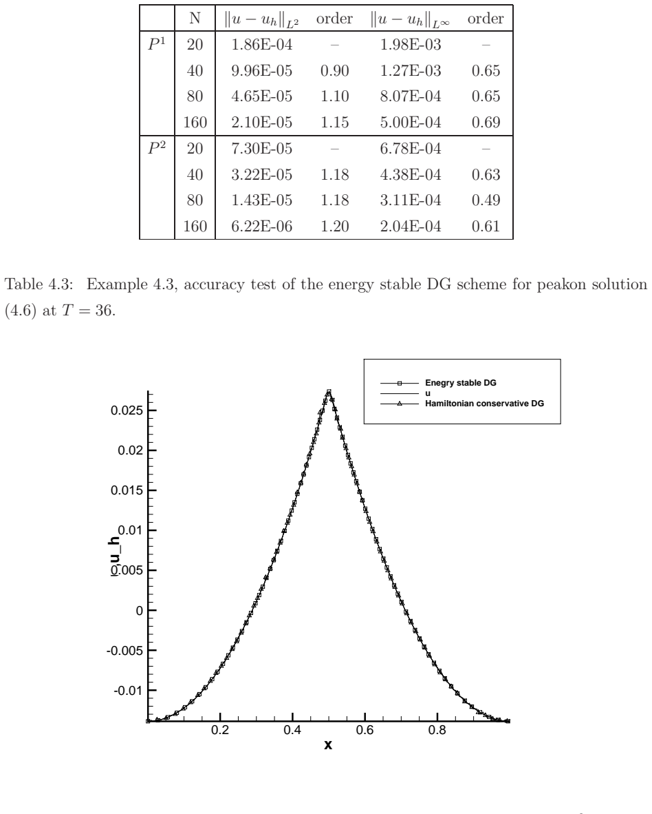
Figures from the paper (3 more)

**Figure 4.3.** Figure 4.3: Example 4.4, the two-cuspon solution u of the OV system (4.7) with the cells N = 320, P 2 elements: The parameters are k1 = 2.0, k2 = 2.6, c = −2.0, ηi0 = −20ki . 23 [PITH_FULL_IMAGE:figures/full_fig_p023_4_3.png]

**Figure 4.4.** Figure 4.4: Example 4.4, the two-cuspon solution q of the OV system (4.7) with the cells N = 320, P 2 elements: The parameters are k1 = 2.0, k2 = 2.6, c = −2.0, ηi0 = −20ki . integration DG scheme for the CD system obtain the profile of solutions of the OV equation via the hodog…

**Figure 4.5.** Figure 4.5: Example 4.4, the two-loop solution u of the OV equation with the cells N = 320, P 2 elements: The parameters are k1 = 1.2, k2 = 1.5, c = 0.0, ηi0 = −20ki . References [1] F. Bassi and S. Rebay. A high-order accurate discontinuous finite element method for the numeric…

Discussion (0). Continue with ORCID to comment.

Reference graph

Works this paper leans on

41 extracted references · 41 canonical work pages

[1]

Bassi and S

F. Bassi and S. Rebay. A high-order accurate discontinuous ﬁn ite element method for the numerical solution of the compressible Navier-Stokes equation s. Journal of Compu- tational Physics, 1997, 131(2): 267-279. 25

work page 1997
[2]

Brunelli and S

J.C. Brunelli and S. Sakovich. Hamiltonian structures for the Ost rovsky-Vakhnenko equation. Communications in Nonlinear Science and Numerical Simulatio n, 2013, 18(1): 56-62

work page 2013
[3]

J. Bona, H. Chen, O. Karakashian and Y. Xing. Conservative, dis continuous Galerkin methods for the generalized Korteweg-de Vries equation. Mathem atics of Computation, 2013, 82(283): 1401-1432

work page 2013
[4]

P.G. Ciarlet. The Finite Element Method for Elliptic Problems. North H olland, 1975

work page 1975
[5]

Cockburn and C.-W

B. Cockburn and C.-W. Shu. The local discontinuous Galerkin meth od for time- dependent convection-diﬀusion systems. SIAM Journal on Numer ical Analysis, 1998, 35(6): 2440-2463

work page 1998
[6]

Cockburn, S.Y

B. Cockburn, S.Y. Lin and C.-W. Shu. TVB Runge-Kutta local proj ection discontinu- ous Galerkin ﬁnite element method for conservation laws III: one-d imensional systems. Journal of Computational Physics, 1989, 84(1): 90-113

work page 1989
[7]

Coclite, J

G.M. Coclite, J. Ridder and N.H. Risebro. A convergent ﬁnite diﬀere nce scheme for the Ostrovsky-Hunter equation on a bounded domain. BIT Numerical M athematics, 2017, 57(1): 93-122

work page 2017
[8]

B.F. Feng, K. Maruno and Y. Ohta. Integrable semi-discretizatio ns of the reduced Os- trovsky equation. Journal of Physics A: Mathematical and Theor etical, 2015, 48(13): 135203

work page 2015

Show all 41 references

[9]

B.F. Feng, K. Maruno and Y. Ohta. A two-component generalizat ion of the reduced Ostrovsky equation and its integrable semi-discrete analogue. Jou rnal of Physics A: Mathematical and Theoretical, 2017, 50(5): 055201

2017
[10]

Gottlieb, C.-W

S. Gottlieb, C.-W. Shu and E. Tadmor. Strong stability-preserv ing high-order time discretization methods. SIAM review, 2001, 43(1): 89-112

2001
[11]

Gui and Y

G. Gui and Y. Liu. On the Cauchy problem for the Ostrovsky equ ation with positive dispersion. Communications in Partial Diﬀerential Equations, 2007, 32(12): 1895-1916

2007
[12]

Grimshaw, K

R.H.J. Grimshaw, K. Helfrich and E.R. Johnson. The reduced Ostr ovsky equation: integrability and breaking. Studies in Applied Mathematics, 2012, 129 (4): 414-436. 26

2012
[13]

J.K. Hunter. Numerical solutions of some nonlinear dispersive wa ve equations. Lect. Appl. Math, 1990, 26: 301-316

1990
[14]

Karakashian and Y.L

O. Karakashian and Y.L. Xing. A posteriori error estimates for conservative local dis- continuous Galerkin methods for the generalized Korteweg-de Vrie s equation. Commu- nications in Computational Physics, 2016, 20(01): 250-278

2016
[15]

Levy, C.-W

D. Levy, C.-W. Shu and J. Yan. Local discontinuous Galerkin met hods for nonlinear dispersive equations. Journal of Computational Physics, 2004, 1 96(2): 751-772

2004
[16]

Linares and A

F. Linares and A. Milan´ es. Local and global well-posedness for the Ostrovsky equation. Journal of Diﬀerential Equations, 2006, 222(2): 325-340

2006
[17]

Y. Liu, D. Pelinovsky and A. Sakovich. Wave breaking in the Ostro vsky-Hunter equa- tion. SIAM Journal on Mathematical Analysis, 2010, 42(5): 1967- 1985

2010
[18]

E.J. Parkes. The stability of solutions of Vakhnenko’s equation. Journal of Physics A: Mathematical and General, 1993, 26(22): 6469

1993
[19]

E.J. Parkes. Explicit solutions of the reduced Ostrovsky equat ion. Chaos, Solitons and Fractals, 2007, 31(3): 602-610

2007
[20]

E.J. Parkes. Some periodic and solitary travelling-wave solutions of the short-pulse equation. Chaos, Solitons and Fractals, 2008, 38(1): 154-159

2008
[21]

Reed and T.R

W.H. Reed and T.R. Hill. Triangular mesh methods for the neutron t ransport equation. Los Alamos Report LA-UR-73-479, 1973

1973
[22]

Ridder and A.M

J. Ridder and A.M. Ruf. A convergent ﬁnite diﬀerence scheme fo r the Ostrovsky-Hunter equation with Dirichlet boundary conditions. BIT Numerical Mathema tics, 2018: 1-22

2018
[23]

Shu and S

C.-W. Shu and S. Osher. Eﬃcient implementation of essentially non -oscillatory shock- capturing schemes. Journal of Computational Physics, 1988, 77 (2): 439-471

1988
[24]

Stepanyants

Y.A. Stepanyants. On stationary solutions of the reduced Ost rovsky equation: Periodic waves, compactons and compound solitons. Chaos, Solitons and Fr actals, 2006, 28(1): 193-204

2006
[25]

Vakhnenko

V.A. Vakhnenko. Solitons in a nonlinear model medium. Journal of Physics A: Mathe- matical and General, 1992, 25(15): 4181. 27

1992
[26]

Vakhnenko and E.J

V.O. Vakhnenko and E.J. Parkes. The two loop soliton solution of t he Vakhnenko equa- tion. Nonlinearity, 1998, 11(6): 1457

1998
[27]

Varlamov and Y

V. Varlamov and Y. Liu. Cauchy problem for the Ostrovsky equa tion. Discrete and Continuous Dynamical Systems-A, 2004, 10(3): 731-753

2004
[28]

Xu and C.-W

Y. Xu and C.-W. Shu. Local discontinuous Galerkin methods for t hree classes of non- linear wave equations. Journal of Computational Mathematics, 20 04: 250-274
[29]

Xu and C.-W

Y. Xu and C.-W. Shu. Local discontinuous Galerkin methods for n onlinear Schr¨ odinger equations. Journal of Computational Physics, 2005, 205(1): 72 -97

2005
[30]

Xu and C.-W

Y. Xu and C.-W. Shu. Local discontinuous Galerkin methods for t wo classes of two- dimensional nonlinear wave equations. Physica D: Nonlinear Phenome na, 2005, 208(1): 21-58

2005
[31]

Xu and C.-W

Y. Xu and C.-W. Shu. Local discontinuous Galerkin methods for t he Kuramoto- Sivashinsky equations and the Ito-type coupled KdV equations. Co mputer Methods in Applied Mechanics and Engineering, 2006, 195(25): 3430-3447

2006
[32]

Xu and C.-W

Y. Xu and C.-W. Shu. Error estimates of the semi-discrete local discontinuous Galerkin method for nonlinear convection-diﬀusion and KdV equations. Comp uter Methods in Applied Mechanics and Engineering, 2007, 196(37-40): 3805-3822

2007
[33]

Xu and C.-W

Y. Xu and C.-W. Shu. Local discontinuous Galerkin methods for h igh-order time- dependent partial diﬀerential equations, Communications in Compu tational Physics, 2010, 7: 1-46

2010
[34]

Y. Xia, Y. Xu and C.-W. Shu. Local discontinuous Galerkin method s for the generalized Zakharov system. Journal of Computational Physics, 2010, 229 (4):1238-1259

2010
[35]

Xia and Y

Y. Xia and Y. Xu. A conservative local discontinuous Galerkin met hod for the Schr¨ odinger-KdV system. Communications in Computational Phys ics, 2014, 15(4): 1091-1107

2014
[36]

Yan and C.-W

J. Yan and C.-W. Shu. A local discontinuous Galerkin method for K dV type equations. SIAM Journal on Numerical Analysis, 2002, 40(2): 769-791

2002
[37]

Yan and C.-W

J. Yan and C.-W. Shu. Local discontinuous Galerkin methods for partial diﬀerential equations with higher order derivatives. Journal of Scientiﬁc Comp uting, 2002, 17(1-4): 27-47. 28

2002
[38]

Zhang and C.-W

Q. Zhang and C.-W. Shu. Error estimates to smooth solutions of Runge–Kutta dis- continuous Galerkin methods for scalar conservation laws. SIAM Jo urnal on Numerical Analysis, 2004, 42(2): 641-666

2004
[39]

Zhang, Y

C. Zhang, Y. Xu and Y. Xia. Local discontinuous Galerkin method s for the µ-Camassa- Holm and µ-Degasperis-Procesi equations. Journal of Scientiﬁc Computing , 79(2019): 1294-1334

2019
[40]

Zhang and Y

Q. Zhang and Y. Xia. Conservative and dissipative local discontin uous Galerkin methods for Korteweg-de Vries type equations. Communications in Computio nal Physics, 2019, 25: 532-563

2019
[41]

Zhang and Y

Q. Zhang and Y. Xia. Discontinuous Galerkin methods for short p ulse type equations via hodograph transformations, arXiv:1907.07842 [math.NA]. 29

1907 arXiv

Pith tools

Reviewed August 14, 2026 · model on record in the stance chip above.

[1] [1]

Bassi and S

F. Bassi and S. Rebay. A high-order accurate discontinuous ﬁn ite element method for the numerical solution of the compressible Navier-Stokes equation s. Journal of Compu- tational Physics, 1997, 131(2): 267-279. 25

work page 1997

[2] [2]

Brunelli and S

J.C. Brunelli and S. Sakovich. Hamiltonian structures for the Ost rovsky-Vakhnenko equation. Communications in Nonlinear Science and Numerical Simulatio n, 2013, 18(1): 56-62

work page 2013

[3] [3]

J. Bona, H. Chen, O. Karakashian and Y. Xing. Conservative, dis continuous Galerkin methods for the generalized Korteweg-de Vries equation. Mathem atics of Computation, 2013, 82(283): 1401-1432

work page 2013

[4] [4]

P.G. Ciarlet. The Finite Element Method for Elliptic Problems. North H olland, 1975

work page 1975

[5] [5]

Cockburn and C.-W

B. Cockburn and C.-W. Shu. The local discontinuous Galerkin meth od for time- dependent convection-diﬀusion systems. SIAM Journal on Numer ical Analysis, 1998, 35(6): 2440-2463

work page 1998

[6] [6]

Cockburn, S.Y

B. Cockburn, S.Y. Lin and C.-W. Shu. TVB Runge-Kutta local proj ection discontinu- ous Galerkin ﬁnite element method for conservation laws III: one-d imensional systems. Journal of Computational Physics, 1989, 84(1): 90-113

work page 1989

[7] [7]

Coclite, J

G.M. Coclite, J. Ridder and N.H. Risebro. A convergent ﬁnite diﬀere nce scheme for the Ostrovsky-Hunter equation on a bounded domain. BIT Numerical M athematics, 2017, 57(1): 93-122

work page 2017

[8] [8]

B.F. Feng, K. Maruno and Y. Ohta. Integrable semi-discretizatio ns of the reduced Os- trovsky equation. Journal of Physics A: Mathematical and Theor etical, 2015, 48(13): 135203

work page 2015