REVIEW 2 major objections 4 minor 41 references
Comparison of time-distance inversion methods applied to SDO/HMI Dopplergrams
T0 review · 2 major / 4 minor · reviewed 2026-08-14 · deepseek-v4-flash
Pith's one-line read The publicly released JSOC sound-speed maps for the quiet Sun are inflated by contamination from the larger-amplitude horizontal flows, while their averaging kernels are not localised at the labelled depths.
desk verdict A careful pipeline comparison that convincingly shows JSOC depth labels are misleading; the cross-talk explanation for the sound-speed amplitude excess is plausible but not directly tested. read the letter →
The pith
A machine-rendered reading of the paper's core claim, the machinery that carries it, and where it could break.
The reading
What carries the argument
The machinery is the multichannel subtractive optimally localised averaging (MC-SOLA) scheme, in which the inversion for horizontal flows, vertical flow, and sound-speed perturbations is performed at once and the cost function includes a term that minimises the integrals of the off-diagonal averaging kernels $K^\alpha_\beta$ for $\alpha \neq \beta$, the cross-talk. The averaging kernels themselves, which connect the inverted estimate to the true subsurface quantities, are the diagnostic objects: their mean depth and vertical extent let the paper quantify how localised each product really is. A JSOC-style regularised least-squares inversion is the counterpoint: its cost function fits travel times and applies smoothing, but the shape of the averaging kernel never enters the solution, so cross-talk cannot be suppressed. Three inversion setups, JSOC-like, JSOC-like target, and JSOC-indicated target, isolate the effect of the target function from the effect of the travel-time set.
What would settle it
Because flow cross-talk should imprint the flow geometry on the sound-speed maps, one could measure the spatial correlation between the JSOC sound-speed maps and the divergence of the JSOC horizontal flow maps: a strong positive correlation would confirm the cross-talk mechanism, while a null correlation would leave the amplitude excess unexplained. Alternatively, run the JSOC-style regularised least-squares inversion on synthetic travel times with zero sound-speed perturbations and known flows; if it returns large sound-speed RMS, cross-talk is directly demonstrated.
Extended reading notes
Core claim
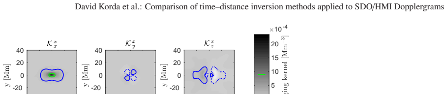
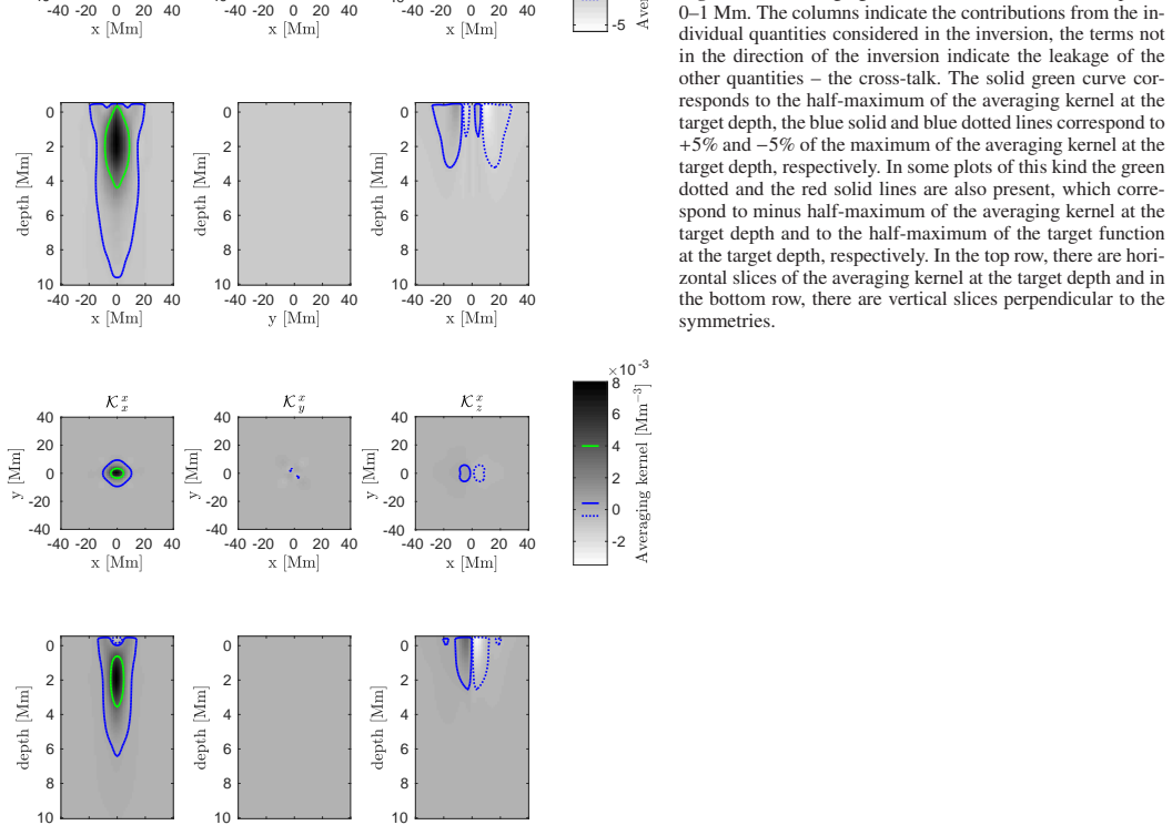
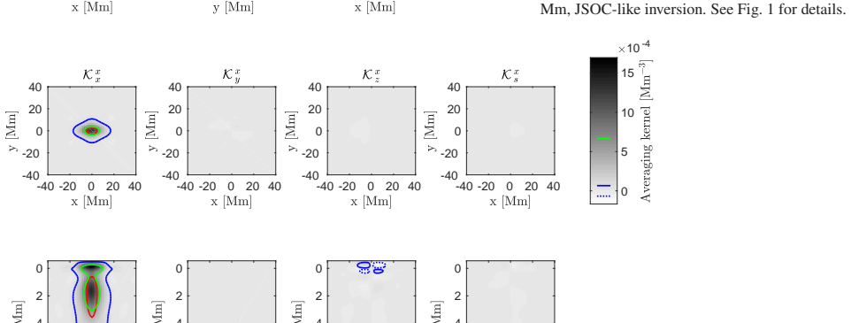
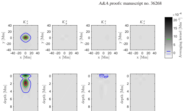
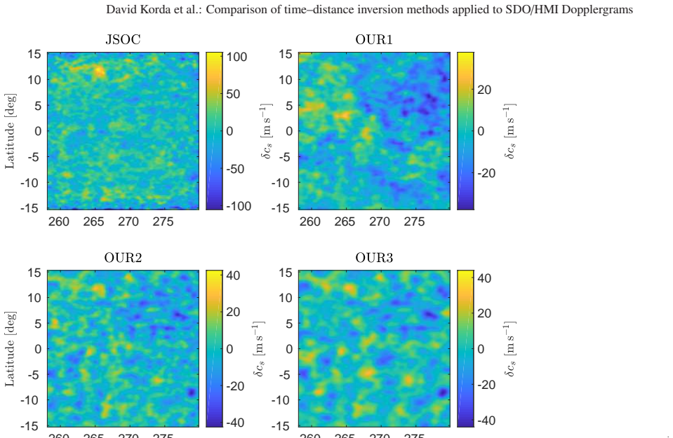
The central claim is that the JSOC sound-speed perturbation products are strongly affected by a high level of cross-talk, which leads to larger amplitudes in the inversions, while the horizontal flow components are faithfully reproduced. Using the JSOC averaging kernels as targets, the independent SOLA pipeline recovers flow maps correlated with JSOC at 0.86-0.94 at shallow depths, but the sound-speed maps show RMS values around $9\text{--}10~\mathrm{m\,s^{-1}}$ against $18~\mathrm{m\,s^{-1}}$ for JSOC, with the best correlation of 0.64 at 2 Mm depth. The authors attribute part of the excess to positively correlated contamination from the flows, consistent with their earlier synthetic-data finding that cross-talk can make up about half of an inverted sound-speed estimate. The same comparison shows that JSOC averaging kernels for the first three indicated depths all peak near 2 Mm and extend from the surface to roughly 4 Mm, so the depth labels in the public products do not correspond to the actual localisation; only the 5-7 Mm map reaches a mean sensitivity near 5.5 Mm.
Load-bearing premise
The load-bearing assumption is that quiet-Sun sound-speed perturbations are genuinely small, roughly an order of magnitude below the horizontal flow amplitudes, as magnetoconvection models predict; if real near-surface sound-speed perturbations are larger than these models say, part or all of the excess amplitude in the JSOC maps could be real signal rather than cross-talk.
Editorial extensions
If this is right
- Users of the public JSOC sound-speed maps should treat the labelled depths as approximate and the amplitudes as upper limits: the maps mix the surface-to-4-Mm layer, and part of their RMS is contamination from the larger-amplitude flows.
- Studies using JSOC flow maps for the horizontal components remain on firmer ground: correlations with the independent pipeline are high (0.86-0.94) at shallow depths, with comparable structure and amplitudes.
- Apparent vertical coherence of near-surface flows across depth bins (correlations of 0.96-0.99 between the top three depth maps) is likely an artefact of the broad, poorly localised averaging kernels rather than evidence for physically coherent depth structure.
- Deep sound-speed and vertical-flow inversions from 24-hour-averaged travel times cannot achieve signal-to-noise above unity; the depth labels for those products give a misleading impression of localisation.
- Combining difference and mean travel-time geometries with ridge-filtered measurements in one inversion lowers both the noise and the cross-talk, so a routine product built this way would be more trustworthy.
Reading between the lines
- If the true quiet-Sun sound-speed perturbations are closer to the upper range allowed by convection simulations, the JSOC excess would be partly signal; the cross-talk explanation could be tested by checking whether the excess amplitude scales with flow amplitude or flow divergence across active and quiet regions.
- The same comparative protocol could be applied to other routinely produced local-helioseismic inversions, such as density or magnetic perturbations, where the regularised least-squares method is used without kernel constraints; cross-talk may be inflating those products too.
- The depth-localisation figures suggest a practical rule for consumers: for a product to be called depth-resolved, the averaging kernel's mean depth should lie within the labelled bin and its width should be smaller than the bin spacing, a criterion the JSOC sound-speed and vertical-flow products do not meet.
- An automated pipeline of the SOLA type could in principle be run at the same cadence as JSOC products, since the added degrees of freedom are a matter of cost-function design rather than new observations.
Signed reviews
Editorial analysis
A structured set of objections, weighed in public.
Referee Report
Summary. The paper compares the standard JSOC time–distance inversion products for horizontal flows and sound-speed perturbations with maps produced by the authors' independent MC-SOLA pipeline applied to the same SDO/HMI Dopplergrams. The authors perform three types of inversions: a JSOC-like inversion using the same travel-time geometries, a JSOC-like-target inversion using a richer set of travel times, and a JSOC-indicated-target inversion using localized Gaussian target functions. They report that horizontal flow maps are well reproduced (correlations 0.82–0.94), while JSOC sound-speed maps have systematically larger RMS amplitudes, which they attribute to cross-talk with the larger-amplitude flows. They also show that the JSOC averaging kernels for the horizontal flows are broad in depth and not localized around the labeled depths, and they argue that this makes the labeled depth structure of the public products misleading. The paper concludes that JSOC inversions are representative of near-surface layers but that the sound-speed amplitudes are likely overestimated through cross-talk.
Significance. If the central conclusion holds, the paper has a direct practical impact: users of the public JSOC time–distance products should not interpret the labeled depths as localized sensitivity depths, and sound-speed amplitudes should be treated with caution. The comparison is genuinely useful because it is an external validation of a widely used data pipeline by an independent inversion code, and it makes use of the actual JSOC averaging kernels for the horizontal flows as target functions. The horizontal-flow reproduction is a solid positive result, and the non-localization of the flow kernels is well documented with quantitative indicators (Tables 1 and 4). The main weakness is that the sound-speed cross-talk attribution, which is the load-bearing claim in the abstract, is not directly tested with JSOC sound-speed averaging kernels and depends on an external assumption about the magnitude of quiet-Sun sound-speed perturbations.
major comments (2)
- [Section 4.2.2 and Conclusions] The abstract and Section 4.2.2 assert that JSOC sound-speed perturbations are 'strongly affected by the high level of the cross-talk' based on the RMS excess and the prior synthetic study Korda & Svanda (2019). However, Section 3.1 reports that averaging kernels were obtained only for the horizontal flows, not for the JSOC sound-speed inversions. The sound-speed-specific cross-talk term, K^{cs}_{flow}, is therefore never computed for the JSOC setup. The observed RMS excess (JSOC 18 m/s vs. OUR2 9 m/s at 2 Mm) could also arise from differences in horizontal averaging width, vertical weighting, or noise between the two pipelines. The paper should either obtain the JSOC sound-speed averaging kernels, present a synthetic test that quantifies the expected cross-talk amplitude for the actual JSOC setup, or revise the claim to state that cross-talk is a plausible but not yet demonstrated explanation.
- [Section 4.2, first paragraph] The interpretation of the larger JSOC sound-speed RMS as contamination presupposes that quiet-Sun sound-speed perturbations are genuinely about an order of magnitude smaller than horizontal flow velocities, citing Rempel (2014) and DeGrave et al. (2014). This assumption is not tested against the data presented in this paper. If the true sound-speed perturbations near 1–3 Mm are larger than those simulations suggest, part or all of the JSOC excess could be real signal. The authors should quantify how sensitive their cross-talk conclusion is to plausible variations in the assumed sound-speed amplitude, or provide an independent observational constraint on that amplitude in the analyzed region.
minor comments (4)
- [Section 1.1] There is a typo in the sentence 'These ocillations are best observed in Doppler shifts' — 'ocillations' should be 'oscillations'.
- [Table 6] In the 'JSOC-indicated target' rows of Table 6 the correlation column is labeled 'corr(OUR2, OUR3)', unlike the 'corr(OUR1, JSOC)' and 'corr(OUR2, JSOC)' used elsewhere. Since the text explains that no JSOC vertical-flow maps are available, this label is understandable, but it should be defined in the table caption for clarity.
- [Section 4.1.1] The statement that the lower RMS in the JSOC-like inversion is 'caused by a larger-than-expected smoothing in the horizontal direction' is plausible but not quantified; giving the horizontal widths or a smoothing comparison of the two kernels would strengthen the point.
- [Section 3.1, Table 2] The near-zero or negative correlations between the JSOC sound-speed maps at 1–3 and 3–5 Mm are noted as unexpected, but no further investigation is offered. A brief comment on whether this could be tested with the authors' pipeline would help the reader interpret the table.
Circularity Check
No circularity: the comparison is an external benchmark against JSOC data, and the one self-cited synthetic study provides independent support rather than a re-entrant input.
full rationale
The paper's claim is comparison-based and empirical: it takes JSOC maps, observed travel times, and JSOC flow averaging kernels as external inputs, then runs its own MC-SOLA inversions against them. The reproduction of the horizontal flows (correlations 0.86–0.94 at shallow depths) is an external benchmark against JSOC products, not a tautology: although the JSOC averaging kernel is used as a target function, the two independent pipelines still process the same observed travel times, so the agreement is informative. The non-localisation conclusion follows directly from JSOC's own kernels via Eq. (7) and Table 1, with the paper explicitly noting that the depth sensitivity for the first three depths is nearly the same and that the JSOC averaging kernel is not localised around the indicated target depth. The sound-speed cross-talk explanation is an inference from three ingredients: the lower RMS in the SOLA maps (9–10 m/s vs 18 m/s at 2 Mm), the positive correlation with the JSOC maps, and the external synthetic result that 'the cross-talk may consist of about one half of the inverted estimate in the case of the inversions for the sound speed' (Korda & Švanda 2019). That last item is a self-citation, but it is an independent synthetic study whose stated assumptions do not include the present measured RMS excess, so it is real evidence and does not make the derivation circular. The paper itself flags the residual uncertainty: 'the cross-talk cannot be evaluated because the inversion setup does not consider contributions from other quantities' (Sec. 4.2.1), and it notes that it obtained averaging kernels 'for the horizontal flows for the first four depths', not for sound speed. These are evidentiary gaps that support a skeptical reading of the amplitude attribution, but they are not cases of an equation reducing to its own input, a fitted parameter relabeled as a prediction, or a load-bearing result imported solely from a self-citation. Therefore no significant circularity is present.
Assumptions & free parameters
free parameters (2)
- SOLA trade-off parameters (mu, nu, epsilon)
- Target function FWHMh and FWHMz =
FWHMh=10 Mm; FWHMz=0.5,1,1,1 Mm
assumptions (4)
- domain assumption Born-approximation sensitivity kernels computed with the Kc3 code correctly model the travel-time response to flows and sound-speed perturbations.
- domain assumption The noise covariance matrix Lambda_ab measured from travel-time data correctly describes realisation noise.
- standard math Model S sound-speed profile is used to convert JSOC fractional delta-cs/cs to absolute m/s units.
- domain assumption Quiet-Sun sound-speed perturbations are small, about an order of magnitude smaller than horizontal flow amplitudes, as in Rempel (2014) and DeGrave et al. (2014).
Cite this review
Pith. "Pith review of Comparison of time-distance inversion methods applied to SDO/HMI Dopplergrams." pith.science (2026). https://pith.science/paper/YOV3UQG3
@misc{pith2026190803950,
  author       = {Pith},
  title        = {Pith review of: Comparison of time-distance inversion methods applied to SDO/HMI Dopplergrams},
  year         = {2026},
  howpublished = {\url{https://pith.science/paper/YOV3UQG3}},
  note         = {Machine review of arXiv:1908.03950}
}
read the original abstract
We compared the results from the JSOC pipeline for horizontal flow components and the perturbations of the speed of sound at set of depths with equivalent results from an independently implemented pipeline using a different time-distance inversion scheme. Our inversion pipeline allows inversion for all quantities at once while allowing minimisation of the crosstalk between them. This gives us an opportunity to discuss the possible biases present in the JSOC data products. For the tests we used the subtractive optimally localised averaging (SOLA) method with a minimisation of the cross-talk. We compared three test inversions for each quantity at each target depth. At first, we used the JSOC setup to reproduce the JSOC results. Subsequently, we used the extended pipeline to improve these results by incorporating more independent travel-time measurements but keeping the JSOC-indicated localisation in the Sun. Finally, we inverted for flow components and sound-speed perturbations using a localisation kernel with properties advertised in the JSOC metadata. We successfully reproduced the horizontal flow components. The sound-speed perturbations are strongly affected by the high level of the cross-talk in JSOC products. This leads to larger amplitudes in the inversions for the sound-speed perturbations. Different results were obtained when a target function localised around the target depth was used. This is a consequence of non-localised JSOC averaging kernels. We add that our methodology also allows inversion for the vertical flow.
Figures

Figures from the paper (12 more)




Reference graph
Works this paper leans on
-
[1]
2016, Living Reviews in Solar Physics, 13, 2
Basu , S. 2016, Living Reviews in Solar Physics, 13, 2
work page 2016
-
[2]
J., Elsworth , Y., New , R., & Serenelli , A
Basu , S., Chaplin , W. J., Elsworth , Y., New , R., & Serenelli , A. M. 2009, , 699, 1403
work page 2009
-
[3]
Birch , A. C. & Gizon , L. 2007, Astronomische Nachrichten, 328, 228
work page 2007
-
[4]
Burston , R., Gizon , L., & Birch , A. C. 2015, , 196, 201
work page 2015
-
[5]
V., et al
Christensen-Dalsgaard , J., Dappen , W., Ajukov , S. V., et al. 1996, Science, 272, 1286
1996
-
[6]
Christensen-Dalsgaard , J., Schou , J., & Thompson , M. J. 1990, , 242, 353
work page 1990
-
[7]
Christensen-Dalsgaard , J., Thompson , M. J., & Gough , D. O. 1989, , 238, 481
work page 1989
-
[8]
Couvidat , S., Birch , A. C., & Kosovichev , A. G. 2006, , 640, 516
work page 2006
Show all 41 references
-
[9]
C., et al
Couvidat , S., Zhao , J., Birch , A. C., et al. 2012, , 275, 357
2012
-
[10]
O., Kosovichev , A
D \"a ppen , W., Gough , D. O., Kosovichev , A. G., & Thompson , M. J. 1991, in Lecture Notes in Physics, Berlin Springer Verlag, Vol. 388, Challenges to Theories of the Structure of Moderate-Mass Stars, ed. D. Gough & J. Toomre , 111
1991
-
[11]
& Jackiewicz , J
DeGrave , K. & Jackiewicz , J. 2015, , 290, 1547
2015
-
[12]
2014, , 788, 127
DeGrave , K., Jackiewicz , J., & Rempel , M. 2014, , 788, 127
2014
-
[13]
Duvall , Jr., T. L. & Birch , A. C. 2010, , 725, L47
2010
-
[14]
Duvall , Jr., T. L. & Gizon , L. 2000, , 192, 177
2000
-
[15]
L., Jefferies , S
Duvall , Jr., T. L., Jefferies , S. M., Harvey , J. W., & Pomerantz , M. A. 1993, , 362, 430
1993
-
[16]
L., Kosovichev , A
Duvall , Jr., T. L., Kosovichev , A. G., Scherrer , P. H., et al. 1997, , 170, 63
1997
-
[17]
M., Duvall , T
Giles , P. M., Duvall , T. L., Scherrer , P. H., & Bogart , R. S. 1997, , 390, 52
1997
-
[18]
M., Duvall , Jr., T
Giles , P. M., Duvall , Jr., T. L., & Scherrer , P. H. 1998, in ESA Special Publication, Vol. 418, Structure and Dynamics of the Interior of the Sun and Sun-like Stars, ed. S. Korzennik , 775
1998
-
[19]
& Birch , A
Gizon , L. & Birch , A. C. 2002, , 571, 966
2002
-
[20]
& Birch , A
Gizon , L. & Birch , A. C. 2004, , 614, 472
2004
-
[21]
C., & Spruit , H
Gizon , L., Birch , A. C., & Spruit , H. C. 2010, , 48, 289
2010
-
[22]
O., Kosovichev , A
Gough , D. O., Kosovichev , A. G., Toomre , J., et al. 1996, Science, 272, 1296
1996
-
[23]
S., Roth , M., et al
Hanasoge , S., Miesch , M. S., Roth , M., et al. 2015, , 196, 79
2015
-
[24]
W., Hill , F., Hubbard , R
Harvey , J. W., Hill , F., Hubbard , R. P., et al. 1996, Science, 272, 1284
1996
-
[25]
& Miesch , M
Hazra , G. & Miesch , M. S. 2018, , 864, 110
2018
-
[26]
C., Gizon , L., et al
Jackiewicz , J., Birch , A. C., Gizon , L., et al. 2012, , 276, 19
2012
-
[27]
Jackiewicz , J., Gizon , L., & Birch , A. C. 2008, , 251, 381
2008
-
[28]
& S vanda , M
Korda , D. & S vanda , M. 2019, , 622, A163
2019
-
[29]
C., & Jefferies , S
Lindsey , C., Braun , D. C., & Jefferies , S. M. 1993, in Astronomical Society of the Pacific Conference Series, Vol. 42, GONG 1992. Seismic Investigation of the Sun and Stars, ed. T. M. Brown , 81
1993
-
[30]
J., Featherstone , N
Nelson , N. J., Featherstone , N. A., Miesch , M. S., & Toomre , J. 2018, , 859, 117
2018
-
[31]
2017, , 607, A120
Passos , D., Miesch , M., Guerrero , G., & Charbonneau , P. 2017, , 607, A120
2017
-
[32]
2014, , 789, 132
Rempel , M. 2014, , 789, 132
2014
-
[33]
H., Bogart , R
Scherrer , P. H., Bogart , R. S., Bush , R. I., et al. 1995, , 162, 129
1995
-
[34]
H., Schou , J., Bush , R
Scherrer , P. H., Schou , J., Bush , R. I., et al. 2012, , 275, 207
2012
-
[35]
H., Bush , R
Schou , J., Scherrer , P. H., Bush , R. I., et al. 2012, , 275, 229
2012
-
[36]
2013, , 775, 7
S vanda , M. 2013, , 775, 7
2013
-
[37]
M., & Ustyugov , S
S vanda , M., Gizon , L., Hanasoge , S. M., & Ustyugov , S. D. 2011, , 530, A148
2011
-
[38]
S., et al
Zhao , J., Couvidat , S., Bogart , R. S., et al. 2012, , 275, 375
2012
-
[39]
G., et al
Zhao , J., Georgobiani , D., Kosovichev , A. G., et al. 2007, , 659, 848
2007
-
[40]
, " * write output.state after.block = add.period write newline
ENTRY address archiveprefix author booktitle chapter edition editor howpublished institution eprint journal key month note number organization pages publisher school series title type volume year label extra.label sort.label short.list INTEGERS output.state before.all mid.sent...
-
[41]
write newline
" write newline "" before.all 'output.state := FUNCTION n.dashify 't := "" t empty not t #1 #1 substring "-" = t #1 #2 substring "--" = not "--" * t #2 global.max substring 't := t #1 #1 substring "-" = "-" * t #2 global.max substring 't := while if t #1 #1 substring * t #2 gl...
Reviewed August 14, 2026 · model on record in the stance chip above.
Discussion (0). Continue with ORCID to comment.