Estimation of the excess mortality in chronic diseases from prevalence and incidence data

Ralph Brinks

REVIEW 4 major objections 6 minor 3 references

Estimation of the excess mortality in chronic diseases from prevalence and incidence data

T0 review · 4 major / 6 minor · reviewed 2026-08-14 · deepseek-v4-flash

Challenge this review Re-run · record.json Download PDF Read on arXiv ↗ Review JSON

Pith's one-line read When prevalence is low, the mortality rate ratio estimated from prevalence and incidence data becomes numerically unstable, so excess mortality should be reported as a rate difference instead.

desk verdict Useful short methods note: convincingly shows R is unstable in claims data, but the case for preferring Δm needs validation. read the letter →

arxiv 1908.04053 v1 pith:Z5YEYNXX submitted 2019-08-12 q-bio.PE stat.ME

Ralph Brinks This is my paper · ORCID

classification q-bio.PEstat.ME

keywords excessmortalityrateratiodifferenceprevalenceincidenceillness-deathmodelinverseproblemclaimsdata

verification ladder T0 review T1 audit T2 compute T3 formal

The pith

A machine-rendered reading of the paper's core claim, the machinery that carries it, and where it could break.

The reading

The paper investigates why estimates of excess mortality in chronic diseases, computed from age-specific prevalence and incidence data, become unreliable at younger ages. Working with German claims data covering about 70 million people and diabetes as the example, it shows that the mortality rate ratio $R=m_1/m_0$ can take impossible negative values below age 55, while the mortality rate difference $\Delta m=m_1-m_0$ remains plausible. The paper points to the ill-posedness of the underlying inverse problem as the likely reason and recommends that excess mortality be reported as the rate difference. The practical payoff would be extending usable excess-mortality estimates to ages below 50, where claims data are increasingly available.

What carries the argument

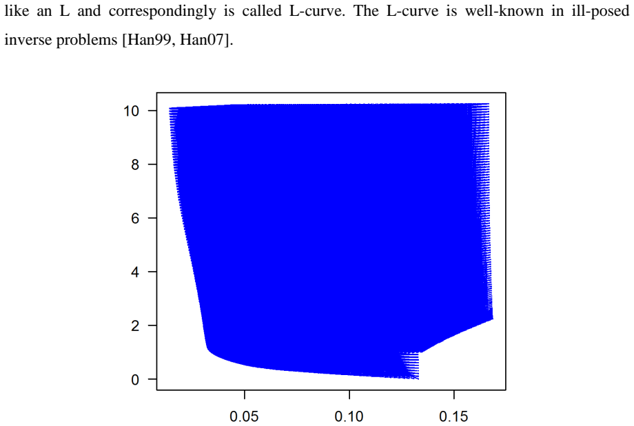
The central object is the illness-death equation for age-specific prevalence $p$, written as $\partial p=(1-p)(i-p\,\Delta m)$ in terms of the rate difference and equivalently in terms of the ratio $R$. Inverting that equation gives the direct estimators $\Delta m=\{i-\partial p/(1-p)\}/p$ and $R=1+(1/p)\{i-\partial p/(1-p)\}/\{m-i+\partial p/(1-p)\}$. The argument turns on the divisor in the $R$ formula: when the combination $m-i+\partial p/(1-p)$ is near zero, small sampling variation in the inputs is amplified, and the outer factor $1/p$ amplifies it further when prevalence is low. The L-curve appearing in the indirect estimation is used as evidence that the difficulty is an ill-posed inverse problem rather than a simple data flaw.

What would settle it

Simulate the illness-death model with known age-specific mortality rates and a known mortality rate ratio $R$ that is constant across age, generate prevalence and incidence from the model, then feed them into Equations (2a) and (2b); if the ratio estimate remains stable below age 55 in that controlled setting, the German-data instability comes from the smoothing or sampling, not from the inverse problem itself.

Watch

Extended reading notes

Core claim

The paper's central claim is that two mathematically equivalent ways of quantifying excess mortality from aggregated data behave very differently in practice. The direct formula for the mortality rate ratio $R$ produces implausible, even negative, estimates for ages below 55 when applied to German diabetes claims data, whereas the direct formula for the rate difference $\Delta m$ gives stable, sensible values. Because a ratio of two positive mortality rates cannot be negative, the negative values signal numerical instability in the inversion, and the paper points to an L-curve typical of ill-posed inverse problems as evidence for that diagnosis. The recommendation is to estimate and report $\Delta m$ rather than $R$ when working from prevalence and incidence data.

Load-bearing premise

The direct estimates assume that logit-transformed prevalence surveys from 2009 and 2015 accurately describe the true temporal change in prevalence over the whole period, with the 2012 incidence curve treated as fixed.

Editorial extensions

If this is right

Epidemiological surveillance based on claims data can report excess mortality down to younger ages if it uses the rate difference instead of the rate ratio.
Studies that currently report only the mortality rate ratio should add the rate difference, because the ratio can be unstable in low-prevalence age groups.
The indirect parameter-fitting approach, judged by its L-curve, offers a way to check whether a direct estimate is trustworthy.
The age range of usable excess-mortality estimates can be extended below the previous practical limit of 50 years, at least for rate differences.

Reading between the lines

Editorial extensions of the paper, not claims the author makes directly.

Not in the paper: the practical trigger for instability is probably low prevalence, because the factor $1/p$ in Equation (2b) amplifies small input errors when $p$ is small; a testable prediction is that chronic conditions with substantial prevalence at young ages will yield stable ratio estimates.
Not in the paper: a regularized or constrained version of the direct ratio estimator, for example one that forces $R\ge 1$ or smooths the denominator before division, might recover a usable ratio; the paper itself stops at recommending $\Delta m$.
Not in the paper: the boundary where $R$ becomes unreliable could be mapped by simulation with known mortality rates, giving applied researchers an explicit age-and-prevalence threshold for when a ratio may safely be quoted.

Share X Bluesky LinkedIn Reddit HN

Signed reviews

No signed human review yet.

Editorial analysis

A structured set of objections, weighed in public.

Desk editor's note, referee report, and a circularity audit.

Desk Editor's Note

read the letter

The paper is a short methods note that does one thing well: Table 1 makes a convincing case that the mortality rate ratio R, estimated from Equations (2a) and (2b) applied to German diabetes claims data, is numerically unstable below age 55, sometimes turning negative. The bootstrap step is a reasonable way to propagate sampling uncertainty, and the paper is honest in showing the implausible R values rather than sweeping them aside. The L-curve from the indirect method is a nice illustration of why the inverse problem is ill-posed, though it is more suggestive than definitive.

What is actually new is modest. The instability of R at young ages was already reported in the cited prior simulation study [Bri19], and Equations (1)–(2) come from [Bri14, Bri16]. The new elements are the real-world application to about 70 million insured Germans and the L-curve picture. That is an incremental extension, not a new technique.

The soft spot is exactly the one flagged in the stress-test note: the recommendation to prefer the rate difference Δm rests on Figure 1 alone. Δm and R share the term A = i − ∂p/(1−p), and both divide by prevalence p, so relative errors in the fitted logit-linear prevalence or in the two-survey time derivative ∂p are amplified at young ages where p is small. R has the extra denominator m − A, which can cross zero and makes R especially fragile, so it is plausible that Δm is better behaved. But plausible is not the same as shown. The paper gives no numeric table for Δm, no coverage checks for the bootstrap intervals, and no comparison with external estimates of diabetes excess mortality. The visual stability of Δm could be an artifact of the smooth 2009–2015 logit-linear fit combined with the constant 2012 incidence. The logit-linear assumption and the time-constant incidence are both load-bearing and unvalidated.

None of this is fatal. The instability result stands. But the central recommendation—that surveillance should prefer Δm—needs more support. A serious referee should ask for sensitivity analyses (e.g., alternative smoothing of prevalence), numeric Δm results with uncertainty, and external validation.

Who gets value from this paper: epidemiologists working with aggregated prevalence/incidence data for chronic disease surveillance. It deserves peer review despite its gaps, because the instability of R is a real finding and the paper honestly raises an important practical question about which estimand to report.

My recommendation: send it to review, but expect or require substantial revision before acceptance. The missing validation of Δm is addressable, not a fundamental flaw.

Referee Report

4 major / 6 minor

Summary. The paper studies estimation of excess mortality in chronic diseases from aggregated age-specific prevalence and incidence data, using German statutory health insurance claims data on diabetes (roughly 70 million people, 2009–2015) as an example. Building on prior work relating the temporal change of age-specific prevalence to incidence and mortality, the author applies two approaches: a direct method using Equations (2a) and (2b), and an indirect method that solves the prevalence PDE for candidate mortality rate ratios R and compares the computed 2015 prevalence with observed values. The main empirical finding is that direct estimates of the mortality rate ratio R from Equation (2b) are numerically unstable and implausible below age 55, including negative values in Table 1, whereas estimates of the mortality rate difference Δm from Equation (2a) appear sensible in Figure 1. The paper concludes that future work should estimate Δm rather than R.

Significance. If the claims are substantiated, the paper would provide a practical recommendation for epidemiological surveillance based on claims data and extend excess-mortality estimation to ages below 50, which is currently considered unreliable. The paper has clear strengths: it uses a large real-world dataset, implements a bootstrap procedure with 2000 replicates, and gives a transparent table showing the instability of direct R estimates. The negative and extreme R values in Table 1 convincingly demonstrate that Equation (2b) is numerically fragile in this application. However, the central recommendation to replace R with Δm rests on the visual stability of Δm in a single example, with no numerical table, no uncertainty diagnostics, no sensitivity analysis for the smoothing assumptions, and no external validation. The paper is therefore more convincing as a cautionary demonstration of instability than as a validated recommendation for a new estimand.

major comments (4)

[Direct methods, Eq. (2a)] The central claim that Δm yields sensible results is not supported by quantitative evidence. Figure 1 shows medians and percentile bands, but no numerical table of Δm is provided, no bootstrap coverage or calibration check is reported, and no comparison is made with external estimates of diabetes excess mortality from the literature. Because Equation (2a) shares the term A = i − ∂p/(1−p) with Equation (2b) and also divides by p, the apparent stability of Δm may be a consequence of the same logit-linear two-survey smoothing and the constant-2012-incidence assumption rather than an intrinsic advantage of Δm. The reader cannot assess whether the authors' recommendation is robust without these additional analyses.
[Direct methods, paragraph 2] The temporal derivative ∂p is estimated from only two prevalence surveys (2009 and 2015) after fitting logit-linear models, and the incidence i is taken from 2012 and treated as fixed over the whole period. This approximation is load-bearing for both Equations (2a) and (2b), yet no sensitivity analysis is presented. For example, the author does not test alternative smoothing functions, alternative knots, or a time-varying incidence rate, nor does the manuscript report the fitted coefficients or residuals of the logit-linear prevalence models. Without such checks, the observed contrast between unstable R and stable Δm could be an artifact of the smoothing, which would undermine the paper's main conclusion.
[Indirect method, Figure 2] The L-curve in Figure 2 is presented as evidence that the inverse problem is ill-posed, and this is used to support the recommendation to prefer Δm. However, the indirect procedure itself has several unexamined assumptions: the choice of knots at ages 30, 60, and 90, the piecewise linear interpolation of log R, and the extrapolation below 30 and above 90. No uncertainty quantification is provided for the indirect estimates, and the L-curve's shape is a heuristic diagnostic, not a validation of the alternative estimand. The connection between the ill-posedness of the indirect inversion and the instability of direct estimates of R would need a more formal argument or at least a simulation study to be load-bearing.
[Results, Table 1] Table 1 shows extreme median R values (e.g., 850 at ages 15–19, −3409 at ages 25–29) and very wide percentile intervals, which clearly indicate instability. However, the bootstrap procedure assumes a binomial error model for prevalence and a Poisson error model for incidence, and the manuscript does not state how the resampling handles the fact that the input data are already smoothed regressions rather than raw counts. If the resampling is applied to the fitted values rather than to the raw data, the uncertainty may be underestimated; if applied to raw data, the regression fits should be repeated within each replicate. The description should be clarified, and the sensitivity of the conclusions to this choice should be discussed.

minor comments (6)

[Figure 2 caption] The caption contains an incomplete citation: the text ends with 'L-curve []' and the reference placeholder is not filled.
[Title and Introduction] There are typographical artifacts in the text, such as 'preval ence' and 'incid ence', which should be corrected.
[References] Reference [Pol01] is cited in the text as '[Pol]' rather than '[Pol01]'; please make the citation consistent.
[Direct methods] The phrase 'sampling uncertainties' is used for variability in claims data, but claims data are not necessarily a random sample; the binomial and Poisson error models are assumptions that should be explicitly justified.
[Indirect method] The manuscript does not report the number of candidate vectors x used to produce Figure 2, nor how the candidate values were generated; this information is needed for reproducibility.
[Conclusion] The conclusion that 'estimates for the rate difference Δm yield sensible results' is stated as a finding, but it is based on one dataset and one figure; adding a numeric summary or a discussion of limitations would make the conclusion more measured.

Circularity Check

0 steps flagged · score 0.0 of 10

No significant circularity: the Δm and R estimates are straightforward inversions of the stated illness-death PDE, not fitted inputs presented as predictions.

full rationale

The paper's central estimates use Eqs. (2a) and (2b), which are algebraic rearrangements of the incidence-prevalence-mortality PDE (1a)-(1b). The inputs are externally reported prevalence, incidence, and general mortality data [Gof17, Fed19]. Estimating Δm and R by solving these equations for the unknown mortality quantities is an inversion of a model, not a definition of the estimand in terms of the estimate; the same data are used because these are estimates, not out-of-sample predictions. The bootstrap resampling (2000 replicates) is an uncertainty analysis, not a fit-then-predict loop. The indirect method fits candidate R values only to display the L-curve diagnostic of ill-posedness; it is not a claim that R is predicted. The self-citations [Bri14, Bri16, Bri18, Bri19, Toe18] provide the model equations and background on the inverse problem, but the current paper's evidence for instability (Table 1, Figure 1, Figure 2) comes from its own application and resampling, so the citations are not load-bearing reductions of the result. The apparent stability of Δm versus instability of R is an empirical finding about the two estimators; possible dependence on the logit-linear smoothing assumption is a validity/correctness concern, not circularity.

Assumptions & free parameters 3 free parameters · 5 assumptions · 0 invented entities

The analysis rests on the illness-death model, the parametric smoothing of prevalence and incidence, the assumed constancy of incidence across the 2009 to 2015 window, and the interpolation and extrapolation rules for R in the indirect method. The smoothing and constancy assumptions are not independently validated, which is why the correctness risk is medium despite the clear instability signal.

free parameters (3)

logit-prevalence regression coefficients (intercept and age slope for 2009 and 2015)
Fitted to the German claims data to obtain smoothed p(a) used in Equations (2a) and (2b); the direct estimates of ∆m and R depend on these curves.
log-incidence regression coefficients (intercept and age slope for 2012)
Fitted to the incidence data by age; used as the i(a) input in Equations (2a) and (2b) and in the indirect PDE solve.
log R at ages 30, 60, 90 = not reported
In the indirect method, these three values are chosen to minimize the squared difference between computed and observed 2015 prevalence; they are fitted parameters, not independently estimated.

assumptions (5)

domain assumption The illness-death model relation (Eq. 1) exactly describes the temporal change of age-specific prevalence.
Taken from [Bri14, Bri16]; the paper uses it without re-derivation or validation against individual-level data.
ad hoc to paper logit(p) is linear in age and the time derivative can be estimated from prevalence surveys in 2009 and 2015 only.
Basis of the direct method's ∂p; no justification or sensitivity analysis is provided for this strong structural assumption.
domain assumption The 2012 incidence i is representative for the whole 2009 to 2015 period and is time-constant.
The incidence from mid-period is used for all calculations, implicitly assuming no temporal trend or cohort effect.
ad hoc to paper The log of the mortality rate ratio R is a straight line in age between 30 and 60 and between 60 and 90, and constant below 30 and above 90.
Used to construct the indirect candidate R(x) for solving the PDE; motivated by Gompertz-Makeham, but the age knots are chosen by the author.
domain assumption The reported general mortality m in 2012 is accurate and applicable.
Taken from the Federal Statistical Office; errors in m would propagate into R estimates.

how reviews work

0 comments

Cite this review

Pith. "Pith review of Estimation of the excess mortality in chronic diseases from prevalence and incidence data." pith.science (2026). https://pith.science/paper/Z5YEYNXX

@misc{pith2026190804053,
  author       = {Pith},
  title        = {Pith review of: Estimation of the excess mortality in chronic diseases from prevalence and incidence data},
  year         = {2026},
  howpublished = {\url{https://pith.science/paper/Z5YEYNXX}},
  note         = {Machine review of arXiv:1908.04053}
}

read the original abstract

Aggregated health data such as claims data from health insurances become more and more available for research purposes. Estimates of excess mortality from prevalence and incidence of a chronic condition have only been possible for ages 50 years and older and have shown to be unstable in younger ages. The aim of this article is to explore the reasons why estimates of excess mortality for younger ages are prone to bias and what can be done to extend the age range to ages below 50 years.

Figures

Figures reproduced from arXiv: 1908.04053 by the authors.

**Figure 2.** Norm of x = (log(R(30), log(R(60)), log(R(90))) (ordinate) over the summed squared differences (pobs – pc(x))2 .(abscissa). Each blue dot corresponds to one pair of x and (pobs – pc(x))2 . The boundary of the blue region to left and to the bottom forms an L-shaped curve called the L-curve []. Conclusion In this manuscript we have described methods to estimate two epidemiological indices for the excess mortality of a… view at source ↗

Discussion (0). Continue with ORCID to comment.

Reference graph

Works this paper leans on

3 extracted references · 3 canonical work pages

[1]

Age- and time-depende nt model of the prevalence of non- communicable diseases and application to dementia i n Germany

[Bri14] Brinks R, Landwehr S. Age- and time-depende nt model of the prevalence of non- communicable diseases and application to dementia i n Germany. Theor Popul Biol. 2014;92:62-8. doi: 10.1016/j.tpb.2013.11.006 [Bri16] Brinks R, Hoyer A, Landwehr S. Surveillance of the incidence of non-communicable diseases (NCDs) with sparse resources: a simulation stu...

work page doi:10.1016/j.tpb.2013.11.006 2014
[2001]

Excess mortal ity for people diagnosed with type 2 diabetes in 2012 - estimates based on claims data f rom 70 million Germans

[Toe18] Tönnies T, Hoyer A, Brinks R. Excess mortal ity for people diagnosed with type 2 diabetes in 2012 - estimates based on claims data f rom 70 million Germans. Nutr Metab Cardiovasc Dis. 2018;28(9):887–91 Contact Ralph Brinks German Diabetes Center Institute for Biometry and Epidemiology University Duesseldorf 40225 Duesseldorf Germany

work page 2012
[2017]

[Han99] Hansen PC, The L-curve and its use in the n umerical treatment of inverse problems, invited chapter, in: P

doi: 10.20364/VA-17.03. [Han99] Hansen PC, The L-curve and its use in the n umerical treatment of inverse problems, invited chapter, in: P. Johnston (Ed.), Computation al Inverse Problems in Electrocardiology, WIT Press, Southampton, 2001: 119–142 [Han07] Hansen PC, Jensen TK, Rodriguez G. An adapt ive pruning algorithm for the discrete L-curve criterion....

work page doi:10.20364/va-17.03

Pith tools

Reviewed August 14, 2026 · model on record in the stance chip above.

[1] [1]

Age- and time-depende nt model of the prevalence of non- communicable diseases and application to dementia i n Germany

[Bri14] Brinks R, Landwehr S. Age- and time-depende nt model of the prevalence of non- communicable diseases and application to dementia i n Germany. Theor Popul Biol. 2014;92:62-8. doi: 10.1016/j.tpb.2013.11.006 [Bri16] Brinks R, Hoyer A, Landwehr S. Surveillance of the incidence of non-communicable diseases (NCDs) with sparse resources: a simulation stu...

work page doi:10.1016/j.tpb.2013.11.006 2014

[2] [2001]

Excess mortal ity for people diagnosed with type 2 diabetes in 2012 - estimates based on claims data f rom 70 million Germans

[Toe18] Tönnies T, Hoyer A, Brinks R. Excess mortal ity for people diagnosed with type 2 diabetes in 2012 - estimates based on claims data f rom 70 million Germans. Nutr Metab Cardiovasc Dis. 2018;28(9):887–91 Contact Ralph Brinks German Diabetes Center Institute for Biometry and Epidemiology University Duesseldorf 40225 Duesseldorf Germany

work page 2012

[3] [2017]

[Han99] Hansen PC, The L-curve and its use in the n umerical treatment of inverse problems, invited chapter, in: P

doi: 10.20364/VA-17.03. [Han99] Hansen PC, The L-curve and its use in the n umerical treatment of inverse problems, invited chapter, in: P. Johnston (Ed.), Computation al Inverse Problems in Electrocardiology, WIT Press, Southampton, 2001: 119–142 [Han07] Hansen PC, Jensen TK, Rodriguez G. An adapt ive pruning algorithm for the discrete L-curve criterion....

work page doi:10.20364/va-17.03