REVIEW 4 major objections 5 minor 59 references
Sampling Distributions of Optimal Portfolio Weights and Characteristics in Low and Large Dimensions
T0 review · 4 major / 5 minor · reviewed 2026-08-14 · deepseek-v4-flash
Pith's one-line read This paper shows that the exact finite-sample joint distribution of estimated optimal portfolio weights and characteristics is captured by a stochastic representation built from five efficient-frontier parameters, and that in high…
desk verdict Sharp exact stochastic representations for optimal portfolios, but the high-dimensional CLT for the GMV variance has a normalization error that must be fixed before anyone builds confidence intervals on it. read the letter →
The pith
A machine-rendered reading of the paper's core claim, the machinery that carries it, and where it could break.
The reading
What carries the argument
The load-bearing mechanism is the efficient-frontier parametrization: every Markowitz-type optimal portfolio is a linear combination of the global minimum-variance portfolio $w_{\mathrm{GMV}} = \Sigma^{-1}\mathbf{1}/(\mathbf{1}^\top\Sigma^{-1}\mathbf{1})$ and the self-financing portfolio $v = Q\mu/(\mu^\top Q\mu)$, where $Q = \Sigma^{-1} - \Sigma^{-1}\mathbf{1}\mathbf{1}^\top\Sigma^{-1}/(\mathbf{1}^\top\Sigma^{-1}\mathbf{1})$, with the scalar function $g$ selecting the specific portfolio. The paper derives the joint stochastic representation of the plug-in estimators of the five determining quantities $V_{\mathrm{GMV}}$, $R_{\mathrm{GMV}}$, $s$, $\theta = Lw_{\mathrm{GMV}}$, and $\eta = Lv$. This representation separates deterministic population matrices from independent standard normal, chi-square, and t components, so samples from the finite-sample distribution can be drawn without recomputing the inverse sample covariance matrix in each simulation, and the high-dimensional limit follows by applying standard central limit results to the independent components.
What would settle it
Simulate returns from a multivariate t distribution with five degrees of freedom, set $n=1000$ and $p/n=0.9$, construct the paper's nominal 95% confidence sets for a non-GMV portfolio such as the expected-utility portfolio, and measure empirical coverage; if coverage falls substantially below 95% while Gaussian-return simulations match, the normality assumption is the load-bearing condition.
Extended reading notes
Core claim
The central claim is Theorem 2.1: for $n>p$ independent $p$-dimensional normal returns, the joint sampling distribution of $(\hat{V}_{\mathrm{GMV}}, \hat{\theta}, \hat{R}_{\mathrm{GMV}}, \hat{s}, \hat{\eta})$ is exactly given by a stochastic representation in which all randomness comes from independent chi-square, normal, and t random variables with scale factors that depend only on the population quantities $V_{\mathrm{GMV}}$, $R_{\mathrm{GMV}}$, $s$, $\theta$, $\eta$, and $LQL^\top$. The paper then shows that every optimal portfolio of the form $w_g = w_{\mathrm{GMV}} + g(R_{\mathrm{GMV}}, V_{\mathrm{GMV}}, s)v$, including the mean-variance, expected-utility, tangency, Sharpe-ratio, minimum-VaR, and minimum-CVaR portfolios, inherits a complete exact sampling distribution through this representation. Under the high-dimensional regime $p/n \to c \in (0,1)$, the scaled estimated weights converge to a multivariate normal distribution with covariance matrix $\Omega_{L,g}$ given in Theorem 4.2, and the paper provides consistent estimators and confidence sets built from these limits.
Load-bearing premise
The derivation is exact only if asset returns are independent multivariate normal with $n>p$, because that assumption makes the sample mean and sample covariance independent and permits the Wishart and inverse Wishart calculations.
Editorial extensions
If this is right
- For any portfolio in the paper's class, exact finite-sample draws of estimated weights and characteristics can be generated from low-dimensional standard distributions, making estimation-risk assessment substantially cheaper than direct Wishart simulation.
- The plug-in estimator of a general optimal portfolio is inconsistent in high dimensions, but the paper's bias-corrected estimators in (4.10)-(4.14) are consistent and can serve as the basis for inference.
- Under $p/n \to c$, the frontier parameter estimators are asymptotically normally distributed with a block-diagonal covariance structure, implying asymptotic independence between certain components such as $\hat{V}_{\mathrm{GMV}}$ and the slope estimator $\hat{s}$.
- The explicit covariance formulas support chi-square-based simultaneous confidence regions and tests on linear combinations of optimal portfolio weights, including a closed-form covariance for the expected-utility portfolio.
- The consistent estimators of the asymptotic covariance matrices allow construction of confidence intervals for optimal portfolio characteristics such as expected return, variance, VaR, and CVaR in the high-dimensional setting.
Reading between the lines
- The paper's own robustness simulations show that heavy-tailed $t$-distributed returns mainly distort $\hat{s}$ and $\hat{V}_{\mathrm{GMV}}$; an extension to elliptical distributions might replace the normal components by t components in the stochastic representation, but this is not claimed in the paper.
- Because the stochastic representation uses only a small number of independent variables regardless of dimension $p$, it could accelerate Bayesian posterior sampling for portfolio weights in large asset universes, although the paper does not develop that connection.
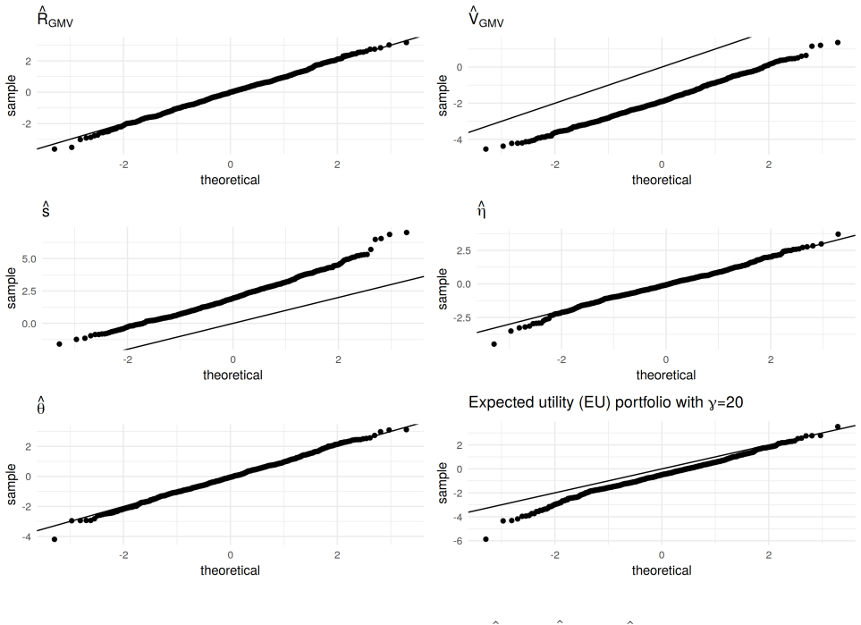
- For concentration ratios close to 1, the normal approximation for $\hat{s}$ is visibly weaker in the simulations, suggesting that a finite-sample correction or a different limit regime for $p/n \to 1$ could be a productive next step.
- The consistent estimator of $LQL^\top$ via $(1-p/n)L\hat{Q}L^\top$ and the resulting estimated covariance matrices open a direct route to power analysis of portfolio-weight tests, which the paper does not pursue.
Signed reviews
Editorial analysis
A structured set of objections, weighed in public.
Referee Report
Summary. The paper characterizes the exact finite-sample joint sampling distribution of the estimated five frontier parameters (GMV variance, GMV weights, GMV expected return, efficient-frontier slope, and self-financing portfolio weights) under i.i.d. multivariate normality, via a stochastic representation (Theorem 2.1). This representation is then used to derive exact stochastic representations for estimated optimal portfolio weights and characteristics (Theorems 3.1 and 3.2), and to obtain high-dimensional central limit theorems under p/n -> c (Theorems 4.1-4.4), together with consistent estimators and confidence regions in Section 4.3. A simulation study in Section 5 assesses the finite-sample quality of the asymptotic approximations and their robustness to t-distributed returns.
Significance. If the stated results were correct, the paper would be a valuable unified treatment: exact finite-sample distributions for a large class of optimal portfolios, an efficient simulation algorithm that avoids inverting the sample covariance matrix in each draw, explicit high-dimensional CLTs, and consistent estimators with confidence regions. The exact finite-sample representation in Theorem 2.1 is a substantial contribution and is derived from standard Wishart, inverse Wishart, and quadratic-form results rather than assumed. The simulation study is extensive and includes a robustness check against heavy-tailed returns. However, I find several load-bearing internal inconsistencies in the displayed formulas: a missing square root in Theorem 3.2, an incorrect asymptotic variance factor in Theorem 4.1(i), an omission of the term mu^T A mu in the asymptotic covariance of the slope estimator, and a structural problem with the claimed covariance-matrix form in Theorem 4.2 for general k. These issues must be resolved before the paper can be accepted.
major comments (4)
- [Section 3, Theorem 3.2] The stochastic representation for hat R_GMV is missing a square root. The proof of Theorem 3.2 shows that, conditional on hat s, hat R_GMV has variance (V_GMV/n)(1 + n/(n-1) hat s), which equals (V_GMV/n)(1 + (p-1)/(n-p+1) psi). Therefore the correct representation is hat R_GMV = R_GMV + sqrt(V_GMV/n) * sqrt(1 + (p-1)/(n-p+1) psi) * z. As printed, Theorem 3.2 states hat R_GMV = R_GMV + sqrt(V_GMV/n)(1 + (p-1)/(n-p+1) psi) z, i.e. the parenthetical factor is not square-rooted. This changes the marginal and joint distributions of all six estimated optimal-portfolio characteristics in Section 3 and would produce incorrect QQ-plots and confidence statements if used directly.
- [Theorem 4.1(i) and proof of Theorem 4.1] The asymptotic coefficient in Theorem 4.1(i) is incorrect. From Theorem 2.1(i), (n-1) hat V_GMV / V_GMV is exactly chi-squared with n-p degrees of freedom, so Var(sqrt(n-p) hat V_GMV) = 2 V_GMV^2 (n-p)^2/(n-1)^2 -> 2(1-c)^2 V_GMV^2. The correct limit is sqrt(n-p)(hat V_GMV - (1-p/n)/(1-1/n) V_GMV) -> sqrt(2)(1-c) V_GMV u1. The printed expression sqrt(2(1-c)) V_GMV u1 has variance 2(1-c) V_GMV^2, a factor 1/(1-c) too large. This is not a typo isolated to one line: the same wrong factor appears in the proof of Theorem 4.1(i) and in the proof of Theorem 4.2 when the u1 term is combined, while Corollary 4.1's (1,1) entry 2 V_GMV^2(1-c)^2 and Theorem 4.4(b)'s 2 V_GMV^2 term both use the corrected coefficient. The printed Theorem 4.1(i) is therefore internally inconsistent with the paper's own exact finite-sample law and with its later covariance formulas. At c=0.9 this overstates the asymptotic variance of hat V_GMV by a factor of 10, which would badly miscalibrate confidence intervals for V_GMV and for any portfolio whose asymptotic distribution enters through g2.
- [Corollary 4.1, entry (4,4)] The displayed variance Xi_{s,s} = 2(c+2s)/(1-c) + 2(s+c)^2/(1-c)^2 does not follow from Theorem 4.1(iv). Since u2, u3, u7 are independent, Theorem 4.1(iv) gives Xi_{s,s} = [2(c+2q)^2 + 4(s-q)]/(1-c) + 2(s+c)^2/(1-c)^2, where q = mu^T A mu and using eta^T (LQL^T)^-1 eta = (s-q)/s^2. The printed expression agrees with this only for a nongeneric value of q, and Assumption (A1) does not restrict q. Consequently the claimed 'direct application' in Corollary 4.1 is not correct as it stands, and the same omission propagates into the Xi_{RVs} matrix used by Theorem 4.3 and hence into the confidence regions of Section 4.3. The authors should re-derive the full covariance matrix from Theorem 4.1 and correct all entries involving mu^T A mu.
- [Theorem 4.2, Eq. (4.7)] The limiting covariance matrix of L hat w_g is not generally of the form a LQL^T + b eta eta^T for k>1. The proof's own expansion contains the independent u3 contribution with coefficient matrix M3 = sqrt(1-c)/(s+c)(g(lam) LQL^T + 2s^2 (g3(lam)/(1-c) - g(lam)/(s+c)) eta eta^T)(LQL^T)^-1/2. The cross term in M3 M3^T is proportional to (LQL^T)^{1/2} eta eta^T (LQL^T)^-1/2 + (LQL^T)^-1/2 eta eta^T (LQL^T)^{1/2}, which for k>1 is not in the linear span of LQL^T and eta eta^T in general; for example, with D = diag(2,1) and eta = (1,1), the cross term cannot be written as aD + b eta eta^T. Since u3 is independent of the other normal variables, this term cannot cancel. Thus Eq. (4.7) is not the correct covariance matrix for general k, and the confidence region in (4.19) is invalid in that setting. The k=1 simulation study would not reveal the problem because every scalar covariance can be represented in the printed form.
minor comments (5)
- [Throughout] There are numerous typos: 'quantites' should be 'quantities', 'On of the issues' should be 'One of the issues', 'pure performance' should be 'poor performance', 'cannot be longer used' should be 'can no longer be used', 'the later property' should be 'the latter property', and 'consequent paper' should be 'subsequent paper'.
- [Proof of Theorem 4.1(i)] The proof uses the notation xi2 for the chi-squared variable driving hat V_GMV, but in Theorem 2.1 xi1 is the chi-squared variable corresponding to hat V_GMV and xi2 corresponds to hat s. Please rename to avoid confusion.
- [Section 4.1, text after Theorem 4.1] The sentence describing the covariance between hat theta and hat R_GMV says it is 'partly determined by the estimated self-financing portfolio hat eta du to the deterministic expression close to u5'; this is hard to parse and should be rewritten.
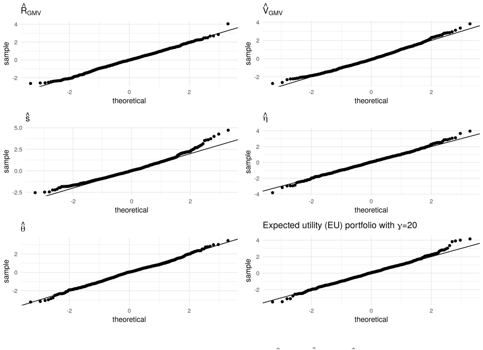
- [Section 5] The discussion says the asymptotic approximation works well for the t(10) scenario, but for hat s and hat V_GMV at c=0.9 the QQ-plots show visible deviations and positive bias. Please state more carefully which quantities are 'well approximated' and which are only approximately so, and note that the bias corrections are deferred to future work.
- [References] Reference [16] is cited as an arXiv preprint; if a published version exists, it should be updated. Also, the reference to 'Bodnar et al. [16, Lemma 5.3]' in Section 4.3 should give the lemma's exact statement for the consistency of (1-p/n) l^T hat Sigma^{-1} l.
Circularity Check
No significant circularity: the exact stochastic representation is derived from Wishart, inverse Wishart, and quadratic-form theory, and the high-dimensional CLT is obtained from that representation rather than assumed.
full rationale
I walked the derivation chain from Section 2 through the appendix. Theorem 2.1 is not assumed or fitted; it is proved from the stated normality assumption xi ~ N_p(mu, Sigma), the Wishart law of (n-1)Sigma-hat, inverse Wishart properties of partitioned matrices, and standard results on linear and quadratic forms in normal variables. The target quantities (V_GMV, theta, R_GMV, s, eta) are expressed in terms of independent chi-square, t, and normal variables after the derivation, not used as inputs. Theorems 3.1 and 3.2 are stated as consequences of Theorem 2.1, which is legitimate deduction rather than circularity. Theorem 4.1 is obtained by applying Slutsky's lemma and asymptotic expansions of chi-square and t variables to the already-derived stochastic representation; Theorem 4.2 then follows by a first-order Taylor expansion of the portfolio-map g, using Theorem 4.1. The simulation section compares the asymptotic approximation against the exact stochastic representation, and the exact representation is itself the derived result, so this comparison is not a fitted-input-called-prediction loop. The paper does invoke the authors' own prior work: Lemma 7.1 uses Theorem 3 of Bodnar and Okhrin (2008), and Section 4.3 cites Lemma 5.3 of Bodnar et al. (2019e) for consistent estimation of l^T Sigma^{-1} l. These are load-bearing in the sense that they provide technical distributional and estimation facts, but they are independent published results with stated assumptions that do not include the paper's target theorems; they are cited as lemmas, not as authority for the main result. There is no step where a quantity is defined in terms of the quantity it is supposed to predict, no parameter is fitted to a subset and then relabeled as a prediction, and no known empirical pattern is merely renamed. The skeptical observation about Theorem 4.1(i) concerns a possible factor error in the asymptotic variance relative to the exact chi-square law; regardless of its correctness, that is an internal consistency/correctness issue, not circularity. I therefore find no significant circularity and assign score 0.
Assumptions & free parameters
assumptions (4)
- domain assumption The return vectors x1,...,xn are independent and multivariate normal with mean µ and covariance Σ, and n > p.
- domain assumption Σ is positive definite, and the matrix M = (L^T, ˜µ, 1)^T has rank k+2.
- domain assumption Assumption (A1): µ^TΣ^{-1}µ, 1^TΣ^{-1}1, and l^TΣ^{-1}l are uniformly bounded away from zero and infinity in p.
- domain assumption For Theorems 4.2 and 4.3, the portfolio-selection function g and characteristic functions h_{g,i} are differentiable with continuous first derivatives.
Cite this review
Pith. "Pith review of Sampling Distributions of Optimal Portfolio Weights and Characteristics in Low and Large Dimensions." pith.science (2026). https://pith.science/paper/ZBVX7763
@misc{pith2026190804243,
  author       = {Pith},
  title        = {Pith review of: Sampling Distributions of Optimal Portfolio Weights and Characteristics in Low and Large Dimensions},
  year         = {2026},
  howpublished = {\url{https://pith.science/paper/ZBVX7763}},
  note         = {Machine review of arXiv:1908.04243}
}
read the original abstract
Optimal portfolio selection problems are determined by the (unknown) parameters of the data generating process. If an investor wants to realise the position suggested by the optimal portfolios, he/she needs to estimate the unknown parameters and to account for the parameter uncertainty in the decision process. Most often, the parameters of interest are the population mean vector and the population covariance matrix of the asset return distribution. In this paper, we characterise the exact sampling distribution of the estimated optimal portfolio weights and their characteristics. This is done by deriving their sampling distribution by its stochastic representation. This approach possesses several advantages, {e.g.} (i) it determines the sampling distribution of the estimated optimal portfolio weights by expressions, which could be used to draw samples from this distribution efficiently; (ii) the application of the derived stochastic representation provides an easy way to obtain the asymptotic approximation of the sampling distribution. The later property is used to show that the high-dimensional asymptotic distribution of optimal portfolio weights is a multivariate normal and to determine its parameters. Moreover, a consistent estimator of optimal portfolio weights and their characteristics is derived under the high-dimensional settings. Via an extensive simulation study, we investigate the finite-sample performance of the derived asymptotic approximation and study its robustness to the violation of the model assumptions used in the derivation of the theoretical results.
Figures

Figures from the paper (1 more)

Reference graph
Works this paper leans on
-
[1]
Adcock, C. (2015). Statistical properties and tests of efficient frontier portfolios. In Quantitative Financial Risk Management, pages 242–269. Wiley Online Library
work page 2015
-
[2]
Aitchison, J. (1964). Confidence-region tests. Journal of the Royal Statistical Society: Series B (Methodological), 26(3):462–476
work page 1964
-
[3]
Alexander, G. J. and Baptista, A. M. (2002). Economic implications of using a mean-var model for portfolio selection: A comparison with mean-variance analysis. Journal of Economic Dynamics and Control, 26(7- 8):1159–1193
work page 2002
-
[4]
Alexander, G. J. and Baptista, A. M. (2004). A comparison of var and cvar constraints on portfolio selection with the mean-variance model. Management science, 50(9):1261–1273. 35
work page 2004
-
[5]
Bai, Z. and Silverstein, J. W. (2010). Spectral Analysis of Large Dimensional Random Matrices. Springer, New York
work page 2010
-
[6]
Bauder, D., Bodnar, R., Bodnar, T., and Schmid, W. (2019). Bayesian estimation of the efficient frontier. Scandinavian Journal of Statistics, 46:802–830
work page 2019
-
[7]
Bodnar, O. and Bodnar, T. (2010). On the unbiased estimator of the efficient frontier. International Journal of Theoretical and Applied Finance, 13(07):1065–1073
work page 2010
-
[8]
Bodnar, T., Dette, H., and Parolya, N. (2019a). Testing for independence of large dimensional vectors. Annals of Statistics, 47(5):2977–3008
work page 2019
Show all 59 references
-
[9]
Bodnar, T., Dmytriv, S., Parolya, N., and Schmid, W. (2019b). Tests for the weights of the global minimum variance portfolio in a high-dimensional setting. IEEE Transactions on Signal Processing, 67(17):4479–4493
2019
-
[10]
K., and Parolya, N
Bodnar, T., Gupta, A. K., and Parolya, N. (2016). Direct shrinkage estimation of large dimensional precision matrix. Journal of Multivariate Analysis, 146:223–236
2016
-
[11]
Bodnar, T., Lindholm, M., Thors´ en, E., and Tyrcha, J. (2018a). Quantile-based optimal portfolio selection. Technical Report 2018:21, Stockholm University
2018
-
[12]
Bodnar, T., Mazur, S., and Okhrin, Y. (2017). Bayesian estimation of the global minimum variance portfolio. European Journal of Operational Research, 256(1):292–307
2017
-
[13]
Bodnar, T., Mazur, S., and Parolya, N. (2019c). Central limit theorems for functionals of large sample covariance matrix and mean vector in matrix-variate location mixture of normal distributions. Scandinavian Journal of Statistics, 46:636–660
2019
-
[14]
Bodnar, T., Okhrin, O., and Parolya, N. (2019d). Optimal shrinkage estimator for high-dimensional mean vector. Journal of Multivariate Analysis, 170:63–79
2019
-
[15]
and Okhrin, Y
Bodnar, T. and Okhrin, Y. (2008). Properties of the singular, inverse and generalized inverse partitioned Wishart distributions. Journal of Multivariate Analysis, 99:2389–2405
2008
-
[16]
Bodnar, T., Okhrin, Y., and Parolya, N. (2019e). Optimal shrinkage-based portfolio selection in high dimensions. arXiv:1611.01958
2019 arXiv
-
[17]
Bodnar, T., Parolya, N., and Schmid, W. (2018b). Estimation of the global minimum variance portfolio in high dimensions. European Journal of Operational Research, 266(1):371–390
2018
-
[18]
and Reiß, M
Bodnar, T. and Reiß, M. (2016). Exact and asymptotic tests on a factor model in low and large dimensions with applications. Journal of Multivariate Analysis, 150:125 – 151
2016
-
[19]
and Schmid, W
Bodnar, T. and Schmid, W. (2008). Estimation of optimal portfolio compositions for gaussian returns. Statistics & Decisions, 26(3):179–201. 36
2008
-
[20]
and Schmid, W
Bodnar, T. and Schmid, W. (2009). Econometrical analysis of the sample efficient frontier. The European journal of finance, 15(3):317–335
2009
-
[21]
Bodnar, T., Schmid, W., and Zabolotskyy, T. (2012). Minimum var and minimum cvar optimal portfolios: estimators, confidence regions, and tests. Statistics & Risk Modeling with Applications in Finance and Insurance, 29(4):281–314
2012
-
[22]
Britten-Jones, M. (1999). The sampling error in estimates of mean-variance efficient portfolio weights. The Journal of Finance, 54:655–671
1999
-
[23]
and Van De Geer, S
B¨ uhlmann, P. and Van De Geer, S. (2011). Statistics for High-Dimensional Data: Methods, Theory and Applications. Springer, Berlin, Heidelberg
2011
-
[24]
and Shen, X
Cai, T. and Shen, X. (2011). High-Dimensional Data Analysis. World Scientific, Singapore
2011
-
[25]
T., Zhang, C.-H., and Zhou, H
Cai, T. T., Zhang, C.-H., and Zhou, H. H. (2010). Optimal rates of convergence for covariance matrix estimation. The Annals of Statistics, 38:2118–2144
2010
-
[26]
DasGupta, A. (2008). Asymptotic Theory of Statistics and Probability. Springer, New York
2008
-
[27]
DeMiguel, V., Garlappi, L., Francisco, N., and Uppal, R. (2009). A generalized approach to portfolio optimization: Improving performance by constraining portfolio norms. Management Science, 55(5):798– 812
2009
-
[28]
Ding, P. (2016). On the conditional distribution of the multivariate t distribution. The American Statistician, 70(3):293–295
2016
-
[29]
and Morris, C
Efron, B. and Morris, C. (1976). Families of minimax estimators of the mean of a multivariate normal distribution. Annals of Statistics, 4:11–21
1976
-
[30]
Fama, E. (1976). Foundations of Finance: Portfolio Decisions and Securities Prices. Basic Books, New York
1976
-
[31]
and Memmel, C
Frahm, G. and Memmel, C. (2010). Dominating estimators for minimum-variance portfolios. Journal of Econometrics, 159:289–302
2010
-
[32]
Givens, G. H. and Hoeting, J. A. (2012). Computational Statistics. John Wiley & Sons
2012
-
[33]
Glombeck, K. (2014). Statistical inference for high-dimensional global minimum variance portfolios. Scandinavian Journal of Statistics, 41:845–865
2014
-
[34]
and Okhrin, Y
Golosnoy, V. and Okhrin, Y. (2007). Multivariate shrinkage for optimal portfolio weights. The European Journal of Finance, 13:441–458
2007
-
[35]
Gupta, A. K. and Nagar, D. K. (2000). Matrix Variate Distributions. Chapman and Hall
2000
-
[36]
K., Varga, T., and Bodnar, T
Gupta, A. K., Varga, T., and Bodnar, T. (2013). Elliptically contoured models in statistics and portfolio theory. Springer. 37
2013
-
[37]
Ingersoll, J. E. (1987). Theory of financial decision making. Rowman & Littlefield
1987
-
[38]
and Ma, T
Jagannathan, R. and Ma, T. (2003). Risk reduction in large portfolios: Why imposing the wrong constraints helps. The Journal of Finance, 58(4):1651– 1683
2003
-
[39]
Jobson, J. (1991). Confidence regions for the mean-variance efficient set: an alternative approach to estimation risk. Review of Quantitative Finance and Accounting, 1(3):235
1991
-
[40]
and Korkie, B
Jobson, J. and Korkie, B. M. (1981). Performance hypothesis testing with the Sharpe and Treynor mea- sures. The Journal of Finance, 36:889–908
1981
-
[41]
and Smith, D
Kan, R. and Smith, D. R. (2008). The distribution of the sample minimum-variance frontier. Management Science, 54(7):1364–1380
2008
-
[42]
and Zhou, G
Kan, R. and Zhou, G. (2007). Optimal portfolio choice with parameter uncertainty. Journal of Financial and Quantitative Analysis, 42(3):621–656
2007
-
[43]
and Turtle, H
Korkie, B. and Turtle, H. J. (2002). A mean-variance analysis of self-financing portfolios. Management Science, 48(3):427–443
2002
-
[44]
and Yang, G
Le Cam, L. and Yang, G. L. (2012). Asymptotics in statistics: some basic concepts. Springer Science & Business Media
2012
-
[45]
Markowitz, H. (1952). Portfolio selection. The Journal of Finance, 7:77–91
1952
-
[46]
Mathai, A. M. and Provost, S. B. (1992). Quadratic forms in random variables: theory and applications. Dekker
1992
-
[47]
and Kempf, A
Memmel, C. and Kempf, A. (2006). Estimating the global minimum variance portfolio. Schmalenbach Business Review, 58:332–348
2006
-
[48]
Muirhead, R. J. (1982). Aspects of Multivariate Statistical Theory. Wiley, New York
1982
-
[49]
and Schmid, W
Okhrin, Y. and Schmid, W. (2006). Distributional properties of portfolio weights. Journal of Econometrics, 134:235–256
2006
-
[50]
and Schmid, W
Okhrin, Y. and Schmid, W. (2008). Estimation of optimal portfolio weights. International Journal of Theoretical and Applied Finance, 11:249–276
2008
-
[51]
Rencher, A. C. (1998). Multivariate statistical inference and applications. Wiley-Interscience
1998
-
[52]
Rubio, F., Mestre, X., and Palomar, D. P. (2012). Performance analysis and optimal selection of large minimum variance portfolios under estimation risk. IEEE Journal of Selected Topics in Signal Processing, 6(4):337–350
2012
-
[53]
Siegel, A. F. and Woodgate, A. (2007). Performance of portfolios optimized with estimation error. Management Science, 53(6):1005–1015. 38
2007
-
[54]
Simaan, M., Simaan, Y., and Tang, Y. (2018). Estimation error in mean returns and the mean-variance efficient frontier. International Review of Economics & Finance, 56:109–124
2018
-
[55]
and Zhou, G
Tu, J. and Zhou, G. (2004). Data-generating process uncertainty: What difference does it make in portfolio decisions? Journal of Financial Economics, 72(2):385–421
2004
-
[56]
Wang, C., Tong, T., Cao, L., and Miao, B. (2014). Non-parametric shrinkage mean estimation for quadratic loss functions with unknown covariance matrices. Journal of Multivariate Analysis, 125:222 – 232
2014
-
[57]
and Siegel, A
Woodgate, A. and Siegel, A. F. (2015). How much error is in the tracking error? The impact of estimation risk on fund tracking error. The Journal of Portfolio Management, 41(2):84–99
2015
-
[58]
Yao, J., Zheng, S., and Bai, Z. (2015). Large Sample Covariance Matrices and High-Dimensional Data Analysis. Cambridge Series in Statistical and Probabilistic Mathematics. Cambridge University Press
2015
-
[59]
and Ando, T
Zellner, A. and Ando, T. (2010). A direct monte carlo approach for bayesian analysis of the seemingly unrelated regression model. Journal of Econometrics, 159:33–45. 39
2010
Reviewed August 14, 2026 · model on record in the stance chip above.
Discussion (0). Continue with ORCID to comment.