REVIEW 4 major objections 4 minor 28 references
Ensemble age inversions for large spectroscopic surveys
T0 review · 4 major / 4 minor · reviewed 2026-08-14 · deepseek-v4-flash
Pith's one-line read The smeared age PDF of a large stellar sample can be inverted to recover the true underlying age distribution, provided the smearing kernel is simulated from mono-age mock catalogues.
desk verdict A genuinely useful inversion method for recovering ensemble age distributions from stacked isochrone-fit PDFs, with self-consistent validation only; the real-data results are suggestive but not yet robust to unquantified model systematics. read the letter →
The pith
A machine-rendered reading of the paper's core claim, the machinery that carries it, and where it could break.
The reading
What carries the argument
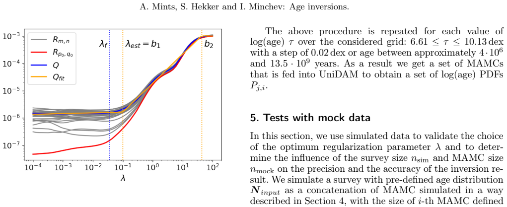
The load-bearing object is the mono-age mock catalogue (MAMC): a simulated set of stars all sharing one $\log(\mathrm{age})$ $\tilde{\tau}$, built from the PARSEC stellar evolution models, with each model star replaced by a small cluster of perturbed copies carrying uncertainties sampled from the base survey, and binned in $\log g$–[Fe/H] to match the survey footprint. Each MAMC is run through the same Bayesian isochrone-fitting pipeline as the real data, yielding the conditional PDF $P(\tau,\tilde{\tau})$ — the smearing kernel. The method turns the integral equation $C(\tau)=\int P(\tau,\tilde{\tau})N(\tilde{\tau})\,d\tilde{\tau}$ into a discretized linear system and solves it with non-negative least squares plus Tikhonov regularization on the first derivative of $N$, the regularization parameter being selected from a piecewise-linear fit to cross-validation residuals. The key identity is that an observed stacked PDF is a mixture of mono-age PDFs, so the mixture weights are precisely the underlying age distribution.
What would settle it
Take a sample of stars from clusters with independently known ages, embed it in a survey-like set, and run the inversion: if the recovered age distribution peaks away from the known cluster ages by more than the quoted confidence intervals, the smearing kernel built from mock catalogues is not the kernel acting on real stars.
Extended reading notes
Core claim
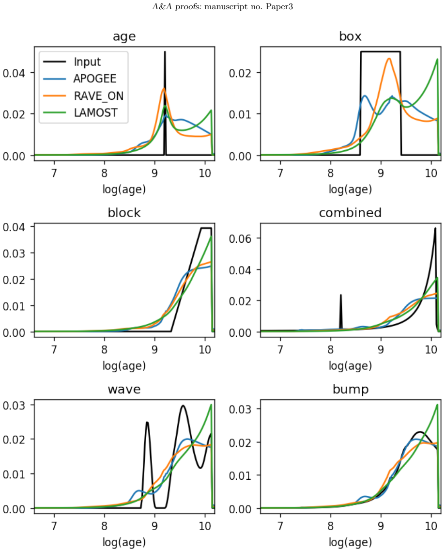
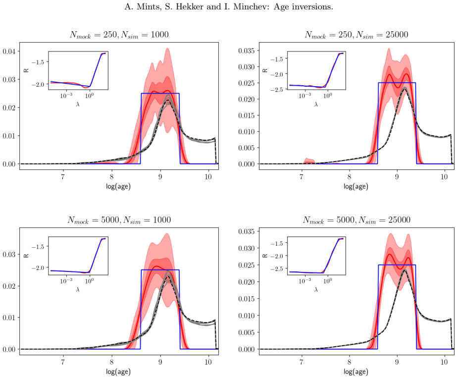
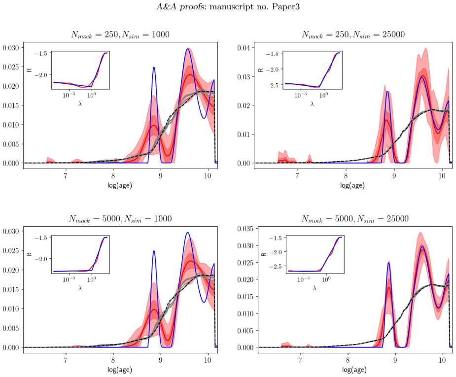
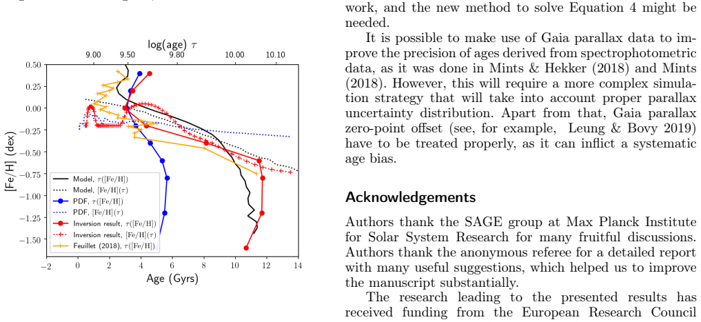
The central claim is that the smeared, stacked $\log(\mathrm{age})$ probability density function of a large stellar ensemble can be inverted to recover the underlying $\log(\mathrm{age})$ distribution $N(\tau)$, as long as the smearing kernel $P(\tau,\tilde{\tau})$ is known. The kernel is built from mono-age mock catalogues: simulated populations of a single age $\tilde{\tau}$, constructed with the same stellar models, the same $\log g$–[Fe/H] distribution, and survey-matched uncertainties as the observed sample, then run through the same Bayesian isochrone-fitting pipeline that produced the observed PDFs. Discretizing $C(\tau)=\int P(\tau,\tilde{\tau})N(\tilde{\tau})\,d\tilde{\tau}$ gives the linear system $C_j=\sum_i P_{j,i}N_i$, solved by non-negative least squares with a Tikhonov smoothness penalty whose strength is set by cross-validation across five survey and mock realizations. On simulated data with known input distributions, the inversion recovers the input age distribution for samples above about $10^3$ stars, whereas the stacked PDF and mean/mode histograms do not. On real surveys, the inversion removes artefacts such as low-age spikes and yields age–metallicity relations close to those from a high-precision local sample and from chemical evolution models. The paper concludes that such an inversion is necessary, not optional, for large ($N>10^3$) stellar samples.
Load-bearing premise
The mono-age mock catalogues must faithfully reproduce how real survey stars get smeared in log(age) by the fitting procedure; if the stellar models or the assigned uncertainties are systematically wrong, the recovered age distribution inherits that wrongness.
Editorial extensions
If this is right
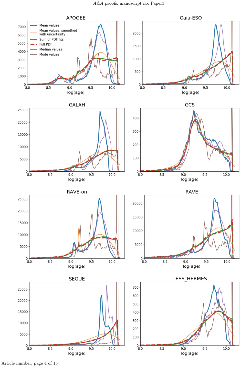
- For any spectroscopic sample of more than about a thousand stars, stacked $\log(\mathrm{age})$ PDFs and mean-age histograms cannot be trusted as age tracers; the inversion must be applied first.
- Age–metallicity relations derived from large, lower-precision surveys can be brought into agreement with high-precision local samples, because the inversion reproduces trends that would otherwise be hidden or distorted by isochrone smearing.
- The recovered full-survey age distributions are bimodal, implying that a single mean age for a survey hides two distinct stellar populations and that splits by metallicity, distance, or sky position are needed to interpret them.
- Because $\tau([\mathrm{Fe/H}])$ and $[\mathrm{Fe/H}](\tau)$ differ unless the two-dimensional age–metallicity distribution is tight, comparisons with chemical evolution models must specify which function is measured; after inversion the two nearly coincide.
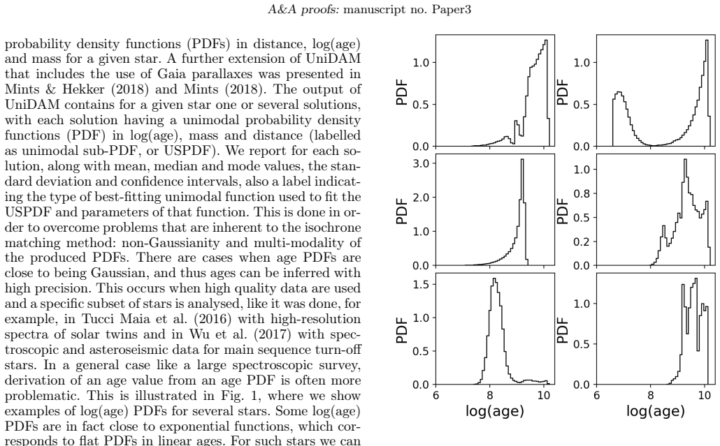
- Spurious low-age spikes in stacked PDFs of old, metal-poor populations disappear after inversion, so samples selected by abundance will show smoother age distributions than the raw PDFs suggest.
Reading between the lines
- The same mixture-deconvolution scheme could be applied to any posterior PDF from Bayesian parameter estimation, such as mass, distance, or initial mass estimates, whenever a smearing kernel can be simulated from mono-value mocks.
- Because the paper finds fractional uncertainty scales roughly as $n_{\mathrm{sim}}^{-0.4} n_{\mathrm{mock}}^{-0.15}$, mock-catalogue sizes beyond a few thousand give diminishing returns; for future million-star surveys, the practical bottleneck is generating enough mocks, so cheaper surrogate kernels for $P(\tau,\tilde{\tau})$ deserve attention.
- An independent cross-check would be to repeat the inversions with a second, independent set of stellar models: wherever the recovered $N(\tau)$ shifts substantially, model systematics rather than survey noise dominate the derived age–metallicity trends.
Signed reviews
Editorial analysis
A structured set of objections, weighed in public.
Referee Report
Summary. The paper presents a method for recovering the underlying log(age) distribution N(τ) of a large stellar sample from the stacked log(age) probability density functions produced by the UniDAM isochrone-fitting pipeline. The central idea is to model the observed stacked PDF C(τ) as a linear superposition of mono-age mock catalogue (MAMC) PDFs P(τ,τ~), leading to the integral equation C(τ)=∫P(τ,τ~)N(τ~)dτ~, discretized and solved with non-negative least squares plus Tikhonov regularization. The regularization parameter is chosen by a cross-validation procedure. The method is tested on simulated surveys built from the same PARSEC/UniDAM pipeline for six input age distributions and varying sample and mock sizes. It is then applied to APOGEE, GALAH, RAVE-on, and LAMOST, including mono-metallicity slices, and the resulting age-metallicity relations are compared with Feuillet et al. (2018) and with chemical evolution models. The paper concludes that such an inversion is necessary to recover underlying age distributions for samples with N>10^3 stars.
Significance. If validated, the method would be a valuable tool for Galactic archaeology, because it directly addresses the well-known bias and multimodality of per-star isochrone ages and provides a way to deconvolve population-level age distributions from large spectroscopic surveys. The mathematical formulation is clear, the non-negativity and regularization choices are standard, and the simulations with known input distributions demonstrate that the method works in an idealized setting. The paper is also honest about several limitations, including the self-consistency of the mock tests and the presence of possible systematic offsets between models and real data. The independent comparison to Feuillet et al. (2018) is a useful external benchmark, although it tests only the mean age-metallicity relation rather than the full recovered distribution. The main weakness is that the load-bearing MAMC kernel is never validated against real data or against an alternative stellar model, so the real-data inversions could be biased.
major comments (4)
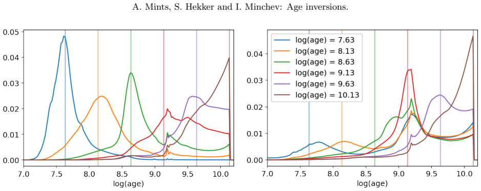
- [Section 4, MAMC construction and Eq. (4)] The kernel P(τ,τ~) is the load-bearing element of Eq. (4), but its construction is not guaranteed to match the real survey. The paper states that within each (logg,[Fe/H]) bin, models are selected with probabilities proportional to the initial-mass-function weight, rather than matching the actual Teff distribution of the survey in that bin. Main-sequence and giant stars contribute very differently to the log(age) PDF, as shown in Fig. 3, so a mismatch in the internal mix within a bin will directly bias P and, through Eq. (4), the recovered N(τ). The authors should either demonstrate that the IMF-weighted sampling reproduces the survey's Teff distribution in each bin or quantify the bias introduced by this approximation.
- [Section 5, tests with mock data] The validation in Section 5 is self-consistent: both the simulated 'observed' survey and the MAMCs are produced from the same PARSEC isochrones, the same uncertainty-assignment procedure, and the same UniDAM pipeline, so any systematic error in the stellar models or in the assumed scatter cancels by construction. The paper acknowledges this in Section 5.3 ('systematic uncertainties are zero by definition') and Section 6.1, but it never quantifies how a mismatch between the true kernel and the assumed MAMC kernel propagates into the recovered N(τ). Given that the central claim is that the method recovers the underlying age distribution of real surveys, the authors should add controlled experiments that perturb the isochrone set, the Teff/logg/[Fe/H] zero-points, or the uncertainty scale, and report the induced changes in the recovered distributions.
- [Sections 6.1 and 6.2, assumption of age independence] The derivation of Eq. (4) assumes that the smearing kernel is the same for all stars of a given true age, independent of their other properties. For the full-survey inversion this requires that age does not depend on logg or [Fe/H] within the sample, an assumption the authors themselves question in Section 6.1. For the mono-metallicity slices in Section 6.2, the same issue persists within each metallicity bin because a magnitude-limited survey selects luminous low-logg stars at larger distances, so the age distribution may vary with logg even at fixed [Fe/H]. The bimodal age distributions and the high-metallicity upturn at [Fe/H]≥+0.2 are left with competing explanations, two of which are artefacts of this assumption. This needs to be modeled or otherwise bounded before the real-data inversions can be interpreted as underlying age distributions.
- [Section 6.3, Eqs. (19) and (20)] Equations (19) and (20) do not define conditional mean ages or mean metallicities as the text claims. For a two-dimensional density C(τ,[Fe/H]), the mean log(age) in a metallicity bin is ∫ τ C(τ,[Fe/H]) dτ / ∫ C(τ,[Fe/H]) dτ, not ∫ C(τ,[Fe/H]) dτ / (τmax−τmin). The same problem affects Eq. (20). If the blue and red curves in Figs. 13–15 were computed with these formulas, they do not measure what the captions claim, and the comparison with Feuillet et al. (2018) and the chemical evolution models is not quantitative. The formulas should be corrected, or the normalization and definition of C(τ,[Fe/H]) should be clarified.
minor comments (4)
- [Eq. (9)] The Toeplitz matrix in Eq. (9) is difficult to read as typeset; the dots and spacing appear garbled. Please typeset it cleanly, for example using \ddots and aligned columns.
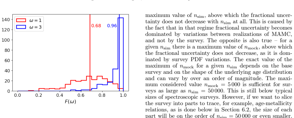
- [Section 5.3] The sentence 'There are no clear trends visible for F(ω) values with nsim and nmock' contains a subject-verb agreement error; it should read 'There are no clear trends visible in F(ω) as a function of nsim and nmock.'
- [Figure 2] The caption of Figure 2 lists line styles, but in the printed version it is not always obvious which line corresponds to the histogram of mean, median, or mode values. A legend or explicitly labeled subpanels would improve readability.
- [Abstract and Section 7] The conclusion that the inversion is 'necessary' to recover underlying age distributions is stronger than what the tests demonstrate. The simulations show that the method works for the considered input distributions and survey sizes, but they do not establish necessity in general. Suggest softening this wording.
Circularity Check
No material circularity: the recovered age distribution is a regularized deconvolution, not a refit of the benchmark data, and the paper explicitly flags the self-consistent mock validation as having zero systematic uncertainty by definition.
full rationale
The central claim is that N(τ) is recovered by solving C(τ)=∫P(τ,τ̃)N(τ̃)dτ̃ (Eq. 4) with P built from mono-age mocks matched to the survey. This is a linear inverse problem; N is not fitted to the external comparison data. The comparison against Feuillet et al. (2018) and against chemical evolution models is an independent sanity check, and the paper does not use those benchmarks as inputs to the inversion. The self-citations (UniDAM from Mints & Hekker 2017; Minchev et al. 2013/2018/2019) are used as tools, motivation, or comparison models, but no load-bearing premise is justified solely by those citations and no uniqueness claim is imported. The strongest potential circularity is the Section 5 mock test: simulated surveys are concatenations of the same MAMC/PARSEC/UniDAM pipeline that defines P, so the inversion recovers an input generated with the same kernel. The paper explicitly acknowledges this: 'all these measurements are done for artificial data, where systematic uncertainties are zero by definition, as simulated and mock catalogues are created from the same set of models' (Section 5.3). This is a closed-loop numerical validation rather than a circular derivation of the real-data result; the real-data conclusions depend on the untested faithfulness of P, which the paper lists as a limitation (Sections 5.3, 6.1, 7). Because the predicted age distributions do not reduce by construction to fitted constants or to the benchmarks, no specific circular step meeting the evidentiary bar can be exhibited. Score 2 reflects the presence of self-citations and a self-consistent validation loop, not load-bearing circularity.
Assumptions & free parameters
free parameters (5)
- Tikhonov regularization parameter lambda =
per-survey, via cross-validation; value not quoted
- Qfit piecewise-linear parameters (a, b1, b2, c, d) =
not quoted
- MAMC size nmock =
250 and 5000 in tests; real-survey values not specified
- Survey split and mock realization count =
5 and 5
- Smoothing scale for chemical evolution model comparison =
2 Gyr in age, 0.1 dex in [Fe/H]
assumptions (5)
- domain assumption PARSEC stellar models and UniDAM isochrone-fitting produce log(age) PDFs that represent the true mapping from physical parameters to observed age PDFs.
- domain assumption The stacked survey PDF is a linear mixture of mono-age population PDFs: C(tau)= integral P(tau,tau_tilde) N(tau_tilde) d tau_tilde.
- ad hoc to paper The true age distribution is smooth, so penalizing the first derivative (Tikhonov regularization) is appropriate.
- domain assumption Within a given inversion, log(age) is independent of log g and [Fe/H].
- standard math Non-negative least squares (Lawson & Hanson 1995) converges to a solution of the regularized linear system.
Cite this review
Pith. "Pith review of Ensemble age inversions for large spectroscopic surveys." pith.science (2026). https://pith.science/paper/5EFXCKDB
@misc{pith2026190804548,
  author       = {Pith},
  title        = {Pith review of: Ensemble age inversions for large spectroscopic surveys},
  year         = {2026},
  howpublished = {\url{https://pith.science/paper/5EFXCKDB}},
  note         = {Machine review of arXiv:1908.04548}
}
read the original abstract
Galactic astrophysics is now in the process of building a multi-dimensional map of the Galaxy. For such a map, stellar ages are the essential ingredient. Ages are however measured only indirectly by comparing observational data with models. It is often difficult to provide a single age value for a given star, as several non-overlapping solutions are possible. We aim at recovering the underlying log(age) distribution from the measured log(age) probability density function for an arbitrary set of stars. We build an age inversion method, namely, we represent the measured log(age) probability density function as a weighted sum of probability density functions of mono-age populations. Weights in that sum give the underlying log(age) distribution. Mono-age populations are simulated so that the distribution of stars on the log g-[Fe/H] plane is close to that of the observed sample. We tested the age inversion method on simulated data, demonstrating that it is capable of properly recovering the true log(age) distribution for a large (N > 103) sample of stars. The method was further applied to large public spectroscopic surveys. For RAVE-on, LAMOST and APOGEE we also applied age inversion to mono-metallicity samples, successfully recovering age-metallicity trends present in higher-precision APOGEE data and chemical evolution models. We conclude that applying an age inversion method as presented in this work is necessary to recover the underlying age distribution of a large (N > 103 ) set of stars. These age distributions can be used to explore for instance age-metallicity relations.
Figures
Figures from the paper (10 more)


Reference graph
Works this paper leans on
-
[1]
Astropy Collaboration, Robitaille, T. P., Tollerud, E. J., et al. 2013, A&A, 558, A33 Bressan,A.,Marigo,P.,Girardi,L.,etal.2012,MNRAS,427,127–145
work page 2013
-
[2]
Casey, A. R., Hawkins, K., Hogg, D. W., et al. 2016, ArXiv e-prints [arXiv:1609.02914]
work page Pith review arXiv 2016
-
[3]
Cutri, R. M. et al. 2014, VizieR Online Data Catalog, 2328
work page 2014
-
[4]
Dalton, G., Trager, S., Abrams, D. C., et al. 2014, in Society of Photo- Optical Instrumentation Engineers (SPIE) Conference Series, Vol. 9147, Ground-based and Airborne Instrumentation for Astronomy V, 91470L de Jong, R. S., Barden, S. C., Bellido-Tirado, O., et al. 2016, in Soci- ety of Photo-Optical Instrumentation Engineers (SPIE) Conference
work page 2014
-
[5]
Dolphin, A. E. 2013, The Astrophysical Journal, 775, 76
work page 2013
-
[6]
K., Bovy, J., Holtzman, J., et al
Feuillet, D. K., Bovy, J., Holtzman, J., et al. 2016, ApJ, 817, 40
work page 2016
-
[7]
K., Bovy, J., Holtzman, J., et al
Feuillet, D. K., Bovy, J., Holtzman, J., et al. 2018, MNRAS, 477, 2326–2348
work page 2018
-
[8]
Hunter, J. D. 2007, Computing In Science & Engineering, 9, 90
2007
Show all 28 references
-
[9]
Lawson, C. L. & Hanson, R. J. 1995, Solving least squares problems, [rev. ed.] edn. (Philadelphia : SIAM)
1995
-
[10]
Leung, H. W. & Bovy, J. 2019, arXiv e-prints, arXiv:1902.08634
2019 arXiv
-
[11]
2015, Research in Astronomy and Astrophysics, 15, 1095
Luo, A.-L., Zhao, Y.-H., Zhao, G., et al. 2015, Research in Astronomy and Astrophysics, 15, 1095
2015
-
[12]
R., Schiavon, R
Majewski, S. R., Schiavon, R. P., Frinchaboy, P. M., et al. 2017, AJ, 154, 94
2017
-
[13]
2016, ArXiv e-prints [arXiv:1609.02822]
Martell, S., Sharma, S., Buder, S., et al. 2016, ArXiv e-prints [arXiv:1609.02822]
2016 arXiv
-
[14]
2018, MNRAS, 481, 1645
Minchev, I., Anders, F., Recio-Blanco, A., et al. 2018, MNRAS, 481, 1645
2018
-
[15]
2013, A&A, 558, A9
Minchev, I., Chiappini, C., & Martig, M. 2013, A&A, 558, A9
2013
-
[16]
W., et al
Minchev, I., Matijevic, G., Hogg, D. W., et al. 2019, MNRAS, 487, 3946
2019
- [17]
-
[18]
& Hekker, S
Mints, A. & Hekker, S. 2017, A&A, 604, A108
2017
-
[19]
& Hekker, S
Mints, A. & Hekker, S. 2018, A&A, 618, A54
2018
-
[20]
& Hekker, S
Mints, A. & Hekker, S. 2019, A&A, 621, A17
2019
-
[21]
Perryman, M. A. C., de Boer, K. S., Gilmore, G., et al. 2001, A&A, 369, 339–363
2001
-
[22]
Queiroz, A. B. A., Anders, F., Santiago, B. X., et al. 2018, MN- RAS[arXiv:1710.09970] Scipy team. 2001, SciPy: Open source scientific tools for Python
2018 arXiv
-
[23]
F., Cutri, R
Skrutskie, M. F., Cutri, R. M., Stiening, R., et al. 2006, AJ, 131, 1163–1183
2006
-
[24]
Soderblom, D. R. 2010, ARA&A, 48, 581–629
2010
-
[25]
Taylor, M. B. 2005, in Astronomical Society of the Pacific Conference
2005
-
[26]
347, Astronomical Data Analysis Software and Systems XIV, ed
Series, Vol. 347, Astronomical Data Analysis Software and Systems XIV, ed. P. Shopbell, M. Britton, & R. Ebert, 29 Tucci Maia, M., Ramírez, I., Meléndez, J., et al. 2016, A&A, 590, A32
2016
-
[27]
2017, Research in As- tronomy and Astrophysics, 17, 5
Wu, Y.-Q., Xiang, M.-S., Zhang, X.-F., et al. 2017, Research in As- tronomy and Astrophysics, 17, 5
2017
-
[28]
2017, The Astrophysical Journal Supplement Series, 232, 2 Article number, page 15 of 15
Xiang, M., Liu, X., Shi, J., et al. 2017, The Astrophysical Journal Supplement Series, 232, 2 Article number, page 15 of 15
2017
Reviewed August 14, 2026 · model on record in the stance chip above.
Discussion (0). Continue with ORCID to comment.