REVIEW 3 major objections 4 minor 32 references
Cataglyphis ant navigation strategies solve the global localization problem in robots with binary sensors
T0 review · 3 major / 4 minor · reviewed 2026-08-14 · deepseek-v4-flash
Pith's one-line read Global localization is possible with only a binary sensor and wheel odometry.
desk verdict A clean proof-of-concept for binary-sensor global localization whose general claim is undercut by in-sample tuning; worth reviewing, but only after held-out maps and ideally a real robot. read the letter →
The pith
A machine-rendered reading of the paper's core claim, the machinery that carries it, and where it could break.
The reading
What carries the argument
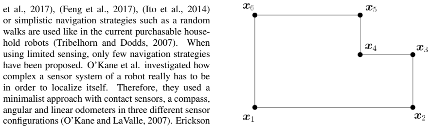
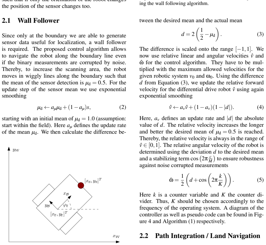
The load-bearing object is the orientation profile $\theta_b(x)$: a piecewise-constant function giving the absolute orientation of each straight boundary segment as a function of distance traveled along the boundary. The robot's odometry path is compressed into dominant points, each representing a segment that is straight within tolerance $e_{\max}$, and from these a second profile $\theta_r$ is built. The algorithm slides $\theta_r$ against vertex-shifted copies of $\theta_b$ and computes the mean absolute correlation error $c_i$; the vertex with the smallest $c_i$ below the trained threshold $c_{\min}$ becomes the first pose estimate. The particle filter then takes over, producing binary-consistent poses by giving each particle weight $\hat{w}$ if its simulated sensor would read the same as the real one and $1-\hat{w}$ otherwise.
What would settle it
Run the same two-stage pipeline on a map with a symmetric or repeated boundary, such as a square or a series of identical straight segments, using the paper's calibrated odometry noise: if a wrong vertex repeatedly gives a correlation error below the threshold and the particle filter converges to a pose far from the true one, the claim that binary sensing plus odometry suffices for global localization in general environments is refuted.
Extended reading notes
Core claim
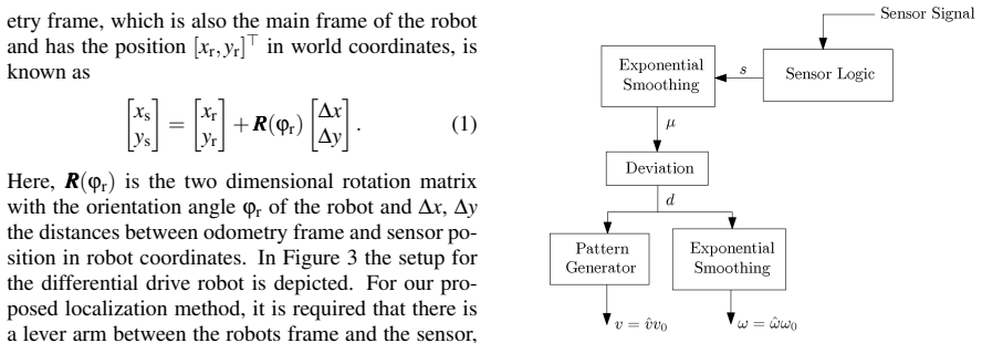
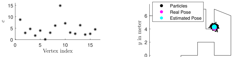
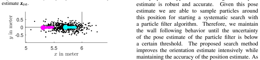
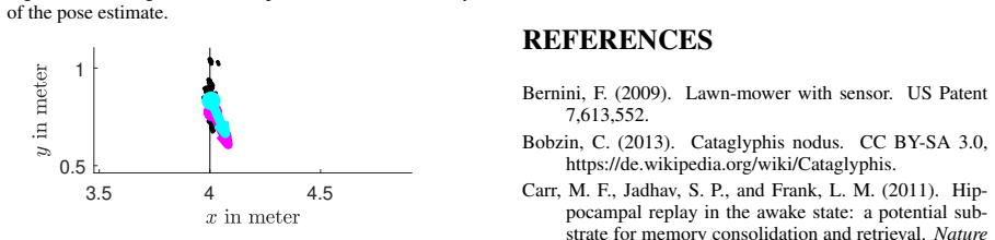
The discovery claimed is that global localization is possible with only odometry plus one binary boundary sensor, provided the problem is split the way Cataglyphis splits it: path integration first, then systematic search. The robot follows the boundary in a wiggly path that keeps the sensor's inside/outside duty cycle near 50%, records the odometry-determined shape of the segment it has traversed, and matches that shape to the map's boundary orientation function. The best-matching vertex, if below a trained correlation threshold, gives a coarse pose in position and heading. Particles are then drawn around that pose and updated by comparing each particle's predicted binary reading with the actual sensor while the robot continues along the wall; the variance of the particles decides when the pose is certain enough to leave the boundary. Simulations in two polygonal maps with noise calibrated to a real lawn mower show position errors around 0.13–0.23 m after the coarse stage and a clear improvement in heading after the particle filter, with 3 of 100 runs failing the accuracy threshold.
Load-bearing premise
The pipeline depends on the boundary's orientation profile being distinctive enough that one vertex stands out below the trained error threshold, and that distinctiveness was only shown on two maps with parameters tuned on those same maps.
Editorial extensions
If this is right
- Lawn mowers with boundary wires can localize without adding any sensor hardware, since the wire signal is exactly the binary measurement used here.
- The two-stage design converts global localization into local refinement, so the particle filter needs far fewer particles than a full global particle filter.
- A robot can leave the boundary to execute a task and re-localize each time it returns to the boundary, because the boundary encounter resets accumulated odometry uncertainty.
- The reported position accuracy near 0.1 m is comparable to a previously published method using a short-range sensor, but achieved with only a cheaper binary sensor.
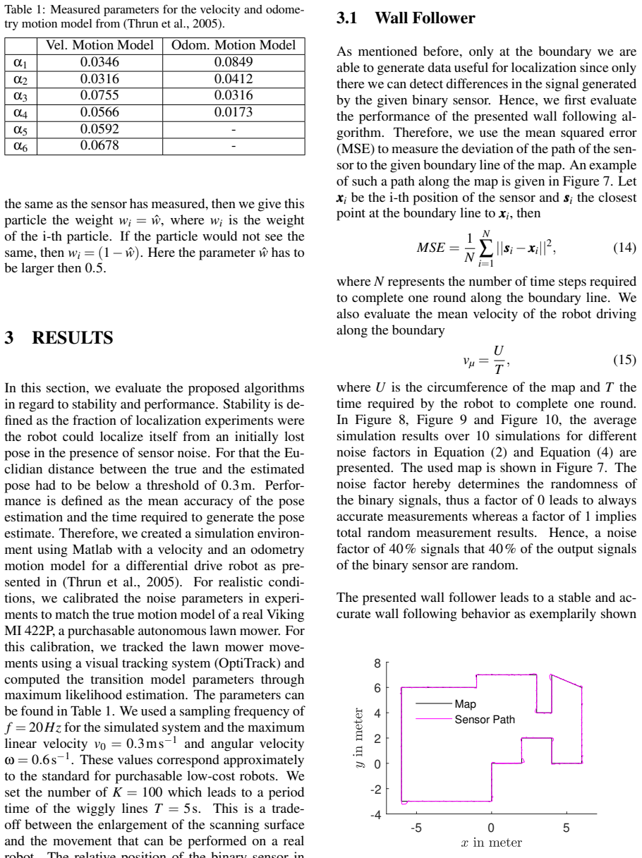
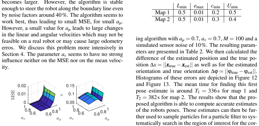
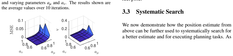
- The wall follower remains stable up to roughly 40% random sensor noise, suggesting tolerance for noisy, low-cost binary hardware.
Reading between the lines
- Editorial inference: in environments with repetitive or symmetric boundary segments—long straight fences, regular polygons, mirrored layouts—the coarse shape match may become ambiguous, and a natural extension is to require confirmation over a longer path or to incorporate segment lengths into the matching score.
- Editorial inference: the trained parameters could be learned online in an unknown environment by treating repeated boundary traversals as a self-supervised calibration loop, which the paper itself flags as an open question.
- Editorial inference: the same two-stage strategy should transfer to other sparse boundary signals, such as mowed/grass moisture sensors or magnetic tape, as long as the sensor has a known lever arm from the odometry frame.
- Editorial inference: the framework suggests a deliberate control policy of periodically returning to the boundary to re-anchor the pose, which could keep long-duration lawn-mowing tasks accurate despite unbounded odometry drift.
Signed reviews
Editorial analysis
A structured set of objections, weighed in public.
Referee Report
Summary. This paper proposes a global localization method for a differential-drive robot equipped only with odometry and a binary sensor that reports whether the sensor is inside or outside a known polygonal boundary. The approach is inspired by Cataglyphis ant navigation and consists of three stages: a wall-following controller that keeps the sensor near the boundary, a land-navigation module that compresses the odometry path into dominant points and matches the resulting orientation profile against the map to obtain an initial vertex-based pose estimate, and a particle filter that samples a Gaussian around that estimate and refines it by continued wall following. The method is evaluated in simulation on two maps, with velocity and odometry noise parameters calibrated from a real lawn mower using a motion-capture system. The reported results show low pose errors after the land-navigation stage and improved orientation estimates after the particle-filter stage, but all algorithm-specific parameters are tuned on the same two maps used for evaluation.
Significance. The two-stage strategy is conceptually attractive: if the land-navigation stage reliably identifies the correct boundary vertex, the particle filter only needs to solve a local problem, potentially making binary-sensor localization feasible on low-cost hardware. Strengths of the paper include a clear algorithmic description, calibration of the motion model to a real platform, and an experimental setup inspired by earlier minimal-sensor localization work. However, the current evidence is limited to two simulated maps with in-sample parameter fitting, no real-robot experiment, and no systematic study of map properties that could cause the initial matching to fail. The contribution is therefore a proof of concept rather than a validated general solution, and the abstract's claim that the method 'can be used in real time on a low-cost robot' goes beyond what is demonstrated.
major comments (3)
- [Section 3.2 (Table 2) & Section 3.3 (Eq. (16))] The evaluation is in-sample. The parameters Lmin, emax, cmin, and Umin are described as 'trained specifically for the given maps' in Section 3.2, and the Gaussian sampling standard deviations in Eq. (16) are set to μΔx + 3σΔx and μΔφ + 3σΔφ using the pose-error statistics measured from the same 100 simulated runs on the same two maps. The reported stability and accuracy are therefore fits to the test environments, not predictions of performance on a new map. This is acknowledged in Section 4 (parameter learning on the fly and real-robot evaluation are listed as open), but the title and abstract still claim a general solution. Please either evaluate with a held-out set of maps after tuning on a training set, or provide a sensitivity analysis over parameter values and a diverse set of maps to show that the method is not critically dependent on per-map tuning.
- [Section 2.2 (Eq. (10)) & Section 3.2] The land-navigation matching step rests on the assumption that the true polygon vertex yields the smallest correlation error ci in Eq. (10) and that this minimum falls below the threshold cmin, while all other vertices produce errors above cmin. This distinctiveness is a property of the map's piecewise orientation function θb(x); it can fail for maps with repeated edges, near-symmetries, or long featureless straight segments, where several vertices generate similar orientation profiles. Because the particle filter samples only a Gaussian around the initial vertex estimate, a wrong match cannot be recovered. The two test maps appear to be generic polygons without such ambiguities, and the paper neither analyzes this condition nor tests maps where it fails. Please add experiments on maps with repeated structure or long straight segments, or characterize the class of maps for which the matching step is guaranteed to succeed.
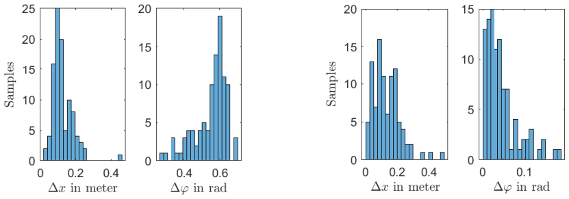
- [Section 3.3] The final results of the complete pipeline are reported incompletely. Section 3 defines stability as the fraction of runs with pose error below 0.3 m, but for the systematic-search stage the text only states that '3 times the particle filter has not found a sufficiently accurate pose estimate' and does not give the overall stability, the mean and standard deviation of the final position and orientation errors across the 100 runs, or the number of particles and the resampling scheme used. Figure 14 shows a histogram, but the text does not state whether it aggregates all runs or a single representative run, and no numerical values are provided. Without these numbers, the claim that the particle filter 'improves the orientation estimate intensively' cannot be verified quantitatively, and the end-to-end success rate after the proposed restart procedure is not measured.
minor comments (4)
- [Section 2.2, Algorithm 2] The prose states that the point S_end−1 is added to the dominant-point set when the line-fit error is acceptable, while Algorithm 2 adds S_end; please reconcile the text with the pseudocode.
- [Section 3.3, Eq. (16)] The notation is confusing: the second argument of the Gaussian is written as μ + 3σ, where μ and σ are the mean and standard deviation of the pose error. Since μ+3σ is a bound rather than a standard deviation, please define the intended covariance matrix explicitly and clarify whether these values are used as variances or standard deviations.
- [Figure 14] The histogram lacks axis labels and units, and it is unclear whether it depicts the errors from all 100 runs or a subset; please add labels and describe the data summarized.
- [Section 4] The comparison with Stavrou and Panayiotou (2012) is qualitative ('similar accuracy') and no quantitative figures are given; since the paper's contribution is specifically the use of a binary sensor, a table with sensor types, map dimensions, and achieved accuracies would strengthen the comparison.
Circularity Check
No significant circularity: the pose estimate is computed by correlation matching against the known map, not from the final pose; the main weakness is in-sample parameter tuning, which is a validity limitation rather than a circular derivation.
full rationale
The derivation chain is self-contained. The initial pose is obtained by minimizing the correlation error in Eq. (10) between the odometry-driven orientation profile θ_r and the map-generated profile θ_b; neither the true pose nor the final particle-filter estimate enters this objective. The particle filter then updates weights from binary measurements and standard motion models, and the wall-follower is an independent control loop. I find no self-definitional equation, no load-bearing self-citation (the two self-citations in the Introduction are motivational), no author-imported uniqueness theorem, and no renamed known result. The only questionable element is statistical: Lmin, emax, cmin and Umin are trained on Map 1 and Map 2 (Table 2), and Eq. (16) sets the PF sampling widths from µ+3σ of the initial-error statistics measured on those same maps in Section 3.2. This makes the reported success rates in-sample; it does not support a claim that the parameters transfer to arbitrary new gardens. However, that is train/test leakage and acknowledged incompleteness, not an equation that reduces the output to the input: the reported pose errors are still produced by the matching and filtering algorithms rather than being equal to the fitted constants. Section 4 explicitly lists learning Lmin, emax, cmin, Umin on the fly and real-robot evaluation as open research, so the paper does not present the two-map results as an out-of-sample prediction. Under the required standard of exhibiting a specific reduction by construction, I therefore find no significant circularity.
Assumptions & free parameters
free parameters (9)
- a_mu =
0.7 in main simulations
- a_v =
0.7 in main simulations
- K =
100
- Lmin =
0.5 for both maps
- emax =
0.01 for both maps
- cmin =
0.2 for Map 1, 0.3 for Map 2
- Umin =
0.5 for Map 1, 0.4 for Map 2
- Particle filter sampling sigma =
mu_delta_x + 3*sigma_delta_x and mu_delta_phi + 3*sigma_delta_phi
- Particle weight w_hat =
not specified, stated as > 0.5
assumptions (5)
- domain assumption A known polygonal boundary map M and a known sensor-to-odometry transform are available.
- domain assumption The robot starts inside the mapped field so that the wall follower can initialize its sensor mean to 1.0.
- domain assumption A lever arm between the robot frame and the binary sensor is required and known.
- domain assumption The odometry and motion model noise parameters calibrated on a real lawn mower transfer to the simulated robot.
- ad hoc to paper The boundary shape is distinctive enough, and the trained parameters reliable enough, that the correlation method finds the correct matching vertex.
Cite this review
Pith. "Pith review of Cataglyphis ant navigation strategies solve the global localization problem in robots with binary sensors." pith.science (2026). https://pith.science/paper/TEHB3ZQP
@misc{pith2026190804564,
  author       = {Pith},
  title        = {Pith review of: Cataglyphis ant navigation strategies solve the global localization problem in robots with binary sensors},
  year         = {2026},
  howpublished = {\url{https://pith.science/paper/TEHB3ZQP}},
  note         = {Machine review of arXiv:1908.04564}
}
read the original abstract
Low cost robots, such as vacuum cleaners or lawn mowers, employ simplistic and often random navigation policies. Although a large number of sophisticated localization and planning approaches exist, they require additional sensors like LIDAR sensors, cameras or time of flight sensors. In this work, we propose a global localization method biologically inspired by simple insects, such as the ant Cataglyphis that is able to return from distant locations to its nest in the desert without any or with limited perceptual cues. Like in Cataglyphis, the underlying idea of our localization approach is to first compute a pose estimate from pro-prioceptual sensors only, using land navigation, and thereafter refine the estimate through a systematic search in a particle filter that integrates the rare visual feedback. In simulation experiments in multiple environments, we demonstrated that this bioinspired principle can be used to compute accurate pose estimates from binary visual cues only. Such intelligent localization strategies can improve the performance of any robot with limited sensing capabilities such as household robots or toys.
Figures

Figures from the paper (14 more)





Reference graph
Works this paper leans on
-
[1]
write newline
" write newline "" before.all 'output.state := FUNCTION fin.entry add.period write newline FUNCTION new.block output.state before.all = 'skip after.block 'output.state := if FUNCTION new.sentence output.state after.block = 'skip output.state before.all = 'skip after.sentence 'output.state := if if FUNCTION not #0 #1 if FUNCTION and 'skip pop #0 if FUNCTIO...
-
[2]
Bernini, F. (2009). Lawn-mower with sensor. US Patent 7,613,552
work page 2009
-
[3]
Bobzin, C. (2013). Cataglyphis nodus. CC BY-SA 3.0, https://de.wikipedia.org/wiki/Cataglyphis
work page 2013
-
[4]
Carr, M. F., Jadhav, S. P., and Frank, L. M. (2011). Hippocampal replay in the awake state: a potential substrate for memory consolidation and retrieval. Nature neuroscience , 14(2):147
work page 2011
-
[5]
Dellaert, F., Fox, D., Burgard, W., and Thrun, S. (1999). Monte carlo localization for mobile robots. In Robotics and Automation, 1999. Proceedings. 1999 IEEE International Conference on , volume 2, pages 1322--1328. IEEE
work page 1999
-
[6]
Erdem, U. M. and Hasselmo, M. (2012). A goal-directed spatial navigation model using forward trajectory planning based on grid cells. European Journal of Neuroscience , 35(6):916--931
work page 2012
-
[7]
Erickson, L. H., Knuth, J., O'Kane, J. M., and LaValle, S. M. (2008). Probabilistic localization with a blind robot. In Robotics and Automation, 2008. ICRA 2008. IEEE International Conference on , pages 1821--1827. IEEE
work page 2008
-
[8]
Feng, L., Bi, S., Dong, M., Hong, F., Liang, Y., Lin, Q., and Liu, Y. (2017). A global localization system for mobile robot using lidar sensor. In 2017 IEEE 7th Annual International Conference on CYBER Technology in Automation, Control, and Intelligent Systems (CYBER) , pages 478--483. IEEE
work page 2017
Show all 32 references
-
[9]
Foster, D. J. and Wilson, M. A. (2006). Reverse replay of behavioural sequences in hippocampal place cells during the awake state. Nature , 440(7084):680
2006
-
[10]
and Carreras, M
Galceran, E. and Carreras, M. (2013). A survey on coverage path planning for robotics. Robotics and Autonomous systems , 61(12):1258--1276
2013
-
[11]
Hess, J., Beinhofer, M., and Burgard, W. (2014). A probabilistic approach to high-confidence cleaning guarantees for low-cost cleaning robots. In Robotics and Automation (ICRA), 2014 IEEE International Conference on , pages 5600--5605. IEEE
2014
-
[12]
Hopfield, J. J. (1982). Neural networks and physical systems with emergent collective computational abilities. Proceedings of the national academy of sciences , 79(8):2554--2558
1982
-
[13]
D., Stachniss, C., and Burgard, W
Ito, S., Endres, F., Kuderer, M., Tipaldi, G. D., Stachniss, C., and Burgard, W. (2014). W-rgb-d: floor-plan-based indoor global localization using a depth camera and wifi. In Robotics and Automation (ICRA), 2014 IEEE International Conference on , pages 417--422. IEEE
2014
-
[14]
and Redish, A
Johnson, A. and Redish, A. D. (2007). Neural ensembles in ca3 transiently encode paths forward of the animal at a decision point. Journal of Neuroscience , 27(45):12176--12189
2007
-
[15]
Lambrinos, D., M \"o ller, R., Labhart, T., Pfeifer, R., and Wehner, R. (2000). A mobile robot employing insect strategies for navigation. Robotics and Autonomous systems , 30(1-2):39--64
2000
-
[16]
and Jung, S
Lee, H. and Jung, S. (2012). Balancing and navigation control of a mobile inverted pendulum robot using sensor fusion of low cost sensors. Mechatronics , 22(1):95--105
2012
-
[17]
L., Battaglia, F
McNaughton, B. L., Battaglia, F. P., Jensen, O., Moser, E. I., and Moser, M.-B. (2006). Path integration and the neural basis of the'cognitive map'. Nature Reviews Neuroscience , 7(8):663
2006
-
[18]
Miller, D. P. and Slack, M. G. (1995). Design and testing of a low-cost robotic wheelchair prototype. Autonomous robots , 2(1):77--88
1995
-
[19]
and Durrant-Whyte, H
Nebot, E. and Durrant-Whyte, H. (1999). Initial calibration and alignment of low-cost inertial navigation units for land vehicle applications. Journal of Robotic Systems , 16(2):81--92
1999
-
[20]
O'Kane, J. M. and LaValle, S. M. (2007). Localization with limited sensing. IEEE Transactions on Robotics , 23(4):704--716
2007
-
[21]
and Nadel, L
O'keefe, J. and Nadel, L. (1978). The hippocampus as a cognitive map . Oxford: Clarendon Press
1978
-
[22]
Pfeiffer, B. E. and Foster, D. J. (2013). Hippocampal place-cell sequences depict future paths to remembered goals. Nature , 497(7447):74
2013
-
[23]
Redish, A. D. et al. (1999). Beyond the cognitive map: from place cells to episodic memory . MIT press
1999
-
[24]
Rueckert, E., Kappel, D., Tanneberg, D., Pecevski, D., and Peters, J. (2016). Recurrent spiking networks solve planning tasks. Nature Publishing Group: Scientific Reports , 6(21142)
2016
-
[25]
and McNaughton, B
Samsonovich, A. and McNaughton, B. L. (1997). Path integration and cognitive mapping in a continuous attractor neural network model. Journal of Neuroscience , 17(15):5900--5920
1997
-
[26]
and Panayiotou, C
Stavrou, D. and Panayiotou, C. (2012). Localization of a simple robot with low computational-power using a single short range sensor. In Robotics and Biomimetics (ROBIO), 2012 IEEE International Conference on , pages 729--734. IEEE
2012
-
[27]
Su, Z., Zhou, X., Cheng, T., Zhang, H., Xu, B., and Chen, W. (2017). Global localization of a mobile robot using lidar and visual features. In Robotics and Biomimetics (ROBIO), 2017 IEEE International Conference on , pages 2377--2383. IEEE
2017
-
[28]
Tanneberg, D., Peters, J., and Rueckert, E. (2019). Intrinsic motivation and mental replay enable efficient online adaptation in stochastic recurrent networks. Neural Networks - Elsevier , 109:67--80. Impact Factor of 7.197 (2017)
2019
-
[29]
Thrun, S., Burgard, W., and Fox, D. (2005). Probabilistic robotics . MIT press
2005
-
[30]
and Dodds, Z
Tribelhorn, B. and Dodds, Z. (2007). Evaluating the roomba: A low-cost, ubiquitous platform for robotics research and education. In ICRA , pages 1393--1399
2007
-
[31]
Wehner, R. (1987). Spatial organization of foraging behavior in individually searching desert ants, cataglyphis (sahara desert) and ocymyrmex (namib desert). In From individual to collective behavior in social insects: les Treilles Workshop/edited by Jacques M. Pasteels, Jean-...
1987
-
[32]
Zhang, J., Lv, H., He, D., Huang, L., Dai, Y., and Zhang, Z. (2017). Discrete bioinspired neural network for complete coverage path planning. International Journal of Robotics and Automation , 32(2)
2017
Reviewed August 14, 2026 · model on record in the stance chip above.
Discussion (0). Continue with ORCID to comment.