REVIEW 3 major objections 5 minor 92 references
A bayesian-like approach to derive chemical abundances in Type-2 Active Galactic Nuclei based on photoionization models
T0 review · 3 major / 5 minor · reviewed 2026-08-14 · deepseek-v4-flash
Pith's one-line read This paper claims that a Bayesian-like grid comparison of optical emission lines reproduces the oxygen and nitrogen abundances of type-2 AGN narrow-line regions found by detailed tailored photoionization models, within the errors.
desk verdict Useful public tool for AGN abundances; validation is a consistency check against the same code family, not an independent test. read the letter →
The pith
A machine-rendered reading of the paper's core claim, the machinery that carries it, and where it could break.
The reading
What carries the argument
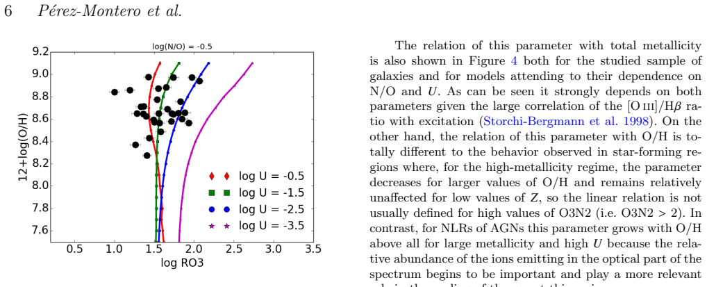
The load-bearing mechanism is the two-stage, chi-squared-weighted Bayesian-like comparison implemented in the HCm code adapted for AGNs: first N/O is set from N2O2 and N2S2, then O/H and log U are set from RO3, N2, O3N2, R23, and O2Ne3. The comparison grid consists of 5,865 Cloudy photoionization models computed for a homogeneous gas slab with density 500 $cm^{-3}$, filling factor 0.1, and a two-component ionizing spectral energy distribution (a big blue bump peaking at 1 Ryd plus a power-law X-ray tail with alpha_ox = -0.8); all abundances are scaled to solar proportions, with nitrogen left free. The grid covers 12+log(O/H) from 6.9 to 9.1, log(N/O) from -2.0 to 0.0, and log U from -4.0 to -0.5, and the code can interpolate the model fluxes by a factor of five in each variable. The restriction to log U > -2.5 avoids the region where the [O ii]/[O iii] versus U relation is double-valued and would degenerate the ionization-parameter solution.
What would settle it
Measure the high-ionization oxygen fraction directly in a few control-sample Seyfert 2s with UV or far-infrared spectroscopy (e.g. [O IV] 25.9 microns, [Ne V] 3426 Angstroms or 14.3/24.3 microns), and compare the total O/H obtained including those ions with the code's predicted ionization-correction factor at the fitted log U; if the model-predicted missing oxygen fraction is contradicted by the observed high-ionization lines, the derived O/H values are systematically biased.
Extended reading notes
Core claim
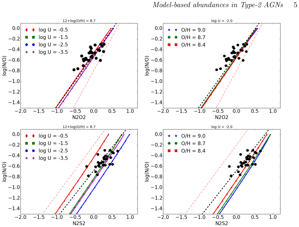
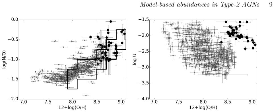
The central discovery is that a Bayesian-like comparison between observed optical emission-line ratios and a precomputed grid of 5,865 photoionization models, run in two stages, recovers the chemical abundances of the narrow-line regions of type-2 AGNs. In the first stage the code derives the nitrogen-to-oxygen ratio from the low-excitation ratios N2O2 and N2S2, which are nearly independent of ionization parameter. In the second stage, with N/O fixed, it derives total oxygen abundance and ionization parameter from RO3, N2, O3N2, R23, and O2Ne3, discarding models with log U below -2.5 to avoid a double-valued relation between [O ii]/[O iii] and U. On the 47-object control sample the method returns O/H values in the range 12+log(O/H) = 8.37 to 9.07 and N/O values in the range log(N/O) = -1.11 to -0.04, agreeing within the errors with the tailored-model determinations of the control sample. The paper interprets the well-known underestimate from the electron-temperature method as an ionization-correction problem: in these high-metallicity, high-U NLRs a large fraction of oxygen occupies ionization stages above O2+ whose optical lines are not measured, so a model-based ionization correction factor is mandatory for total abundances from optical spectra.
Load-bearing premise
The load-bearing premise is that the narrow-line region is effectively a single homogeneous gas slab at density 500 $cm^{-3}$ with a fixed two-component ionizing spectrum, and that the oxygen missing from optical lines really is in higher, unobserved ionization stages; if that ionization correction is wrong, the total O/H values would be systematically biased even though the Bayesian fit appears internally consistent.
Editorial extensions
If this is right
- Large optical surveys of type-2 AGNs can now be processed automatically with the same Bayesian grid code, yielding O/H, N/O, and log U with uncertainties even when the auroral line [O III] lambda4363 or the blue [O II] lambda3727 line is missing.
- Abundances of AGN narrow-line regions and star-forming galaxies can be placed on a common model-based scale, because the same Bayesian-like code has already been applied to H II regions.
- The electron-temperature method's systematically low AGN metallicities should be read as evidence for a large unobserved high-ionization oxygen fraction, not as a contradiction with photoionization models; metallicity- and U-dependent ionization corrections are required.
- The sample's high O/H with N/O increasing toward high metallicity, though with large scatter, supports secondary nitrogen production in these systems and warns against calibrating metallicity from [N II] lines without an independent N/O constraint.
- Because the derived log U values are roughly 1.5 dex higher than in star-forming galaxies at the same metallicity, ionization parameter must be treated separately when comparing AGN and star-forming samples.
Reading between the lines
- If the missing-ionization interpretation is correct, optical-only AGN surveys should adopt a metallicity- and U-dependent ionization-correction factor rather than a constant offset; the paper demonstrates the need in model space but does not publish a closed-form correction formula.
- The double-valued [O ii]/[O iii] versus U relation implies that log U cannot be uniquely derived from strong-line ratios in this regime; the code's choice to keep only the upper branch (log U > -2.5) could hide a population of lower-excitation NLRs, a hypothesis testable with independent indicators such as [Ne V]/[Ne III].
- The same grid-based Bayesian approach should extend to rest-frame UV and mid-infrared line sets, where the supposedly missing high-ionization oxygen ions become directly observable; a successful check there would turn the paper's main assumption into a verified prediction.
- The new linear relations between log(N/O) and N2O2 or N2S2 derived for AGN NLRs could be used as quick empirical N/O estimators for large samples, though their scatter around the control-sample values (roughly 0.12-0.13 dex) sets the precision floor.
Signed reviews
Editorial analysis
A structured set of objections, weighed in public.
Referee Report
Summary. This manuscript presents an adaptation of the public Hii-Chi-mistry code (HCm) to the narrow-line regions of type-2 AGNs. The authors build a grid of 5,865 Cloudy photoionization models spanning 12+log(O/H)=6.9-9.1, log(N/O)=-2.0-0.0, and log U=-4.0 to -0.5 under fixed density (500 cm^-3), filling factor (0.1), and a two-component SED with alpha_ox=-0.8. The code first estimates N/O from the N2O2 or N2S2 ratios, then constrains O/H and U from optical ratios (RO3, N2, O3N2, R23, O2Ne3), restricting log U to > -2.5 to avoid the double-valued [O ii]/[O iii] branch. Applied to 47 Seyfert 1.9/2 galaxies from Dors et al. (2017), the method returns 12+log(O/H)=8.37-9.07, log(N/O)=-1.11 to -0.04, and log U=-2.42 to -1.27, in nominal agreement with the tailored-model abundances of Dors et al. (2017). The paper also shows that the Te-method O^+ + O^2+ ionic abundances fall roughly 0.7 dex below the model total O/H, attributes this to unobserved higher-ionization oxygen, and tests sensitivity to density and alpha_ox.
Significance. If the method is accurate, it would be a convenient, reproducible tool for abundance measurements in large AGN samples and would support the conclusion that Seyfert 2 NLRs are metal-rich, with secondary nitrogen production and high ionization parameters. Strengths of the manuscript include the public release of the code, explicit Monte Carlo uncertainty propagation, a transparent grid, and a fair discussion of the double-valued excitation diagnostics. The principal weakness is that the only quantitative validation uses Dors et al. (2017), whose tailored models share the Cloudy code, the same SED prescription, and an author with the present paper; the agreement therefore validates the numerical inversion but not the physical ionization correction factor that carries the main abundance result. The N/O residual pattern in Table 1 also needs explanation before the "agreement within errors" claim can be accepted in full. With these points addressed, the paper would be a useful methodological contribution.
major comments (3)
- [§4.2 / §4.4] The validation is not independent. Both the new grid and the Dors et al. (2017) control abundances are computed with Cloudy, adopt largely the same SED and homogeneous-slab geometry, and share authorship, so the reported agreement mainly checks that a grid inversion can reproduce tailored fits within the same model family. The physically important claim, that the 0.7 dex deficit of the Te-method O^+ + O^2+ abundances is an ionization correction to total O/H, is exactly the kind of model-dependent step that this comparison cannot test. I request an external validation (e.g., infrared or ultraviolet oxygen lines, X-ray constraints, or an independent photoionization code with different atomic data) or at least a quantitative exploration of matter-bounded geometries and SED variations to show that the derived O/H is not a common bias of the shared assumptions.
- [§3.2.1 / Table 1] The reported N/O residuals are internally inconsistent. The direct N2O2 and N2S2 calibrations against the same Dors et al. (2017) sample give mean offsets of +0.07 and +0.05 dex, but the all-lines solution in Table 1 has a mean residual of +0.23 dex with a scatter of 0.19 dex, and the residual changes non-monotonically with the line set (+0.12 for [O iii]a, [O iii]n, [N ii], [S ii]; -0.11 for [O iii]n, [N ii], [S ii]). Since the code fixes N/O from N2O2/N2S2 before deriving O/H, the origin of this roughly 0.2 dex offset should be explained; as written, it weakens the claim that the method is consistent and independent of the input line set.
- [§3.2.2 / Fig. 13] The decision to discard models with log U < -2.5 is implemented before comparing with the data, and Figure 13 shows that when the full grid is allowed many objects fall in the turnover region that has no models, so the restriction is effectively an assumption rather than a result. Because the abstract emphasizes that the derived log U values are much larger than in star-forming objects, the authors should demonstrate that this conclusion is robust to the branch choice, for example by testing an independent U diagnostic or by reporting how many objects would move to low-log U solutions without the restriction.
minor comments (5)
- [Throughout] The phrase "bayesian-like" is used throughout, but equations (1), (7), and (8) define weighted means with weights 1/chi^2 and no priors or normalization are specified; please either define the probabilistic interpretation or use a less committal term.
- [§3.1] The sentence stating that a density of 500 cm^-3 is "about the maximum value found by Dors et al. (2014)" is incomplete and should be reworded with the relevant reference and a brief justification for choosing the maximum value.
- [Abstract / §4.5] There are typographical errors that should be corrected, including "consistent wit" in the abstract, "more deepley studied" in Section 4.1, and "hte" in Section 4.2.
- [Fig. 14] The solid model lines for different values of U in Figure 14 are not identified in the caption; a legend or line labels are needed for the comparison with the black circles.
- [§4.2] The statement that there are no degeneracies between metallicity and the optical ratios for log U > -2.5 is strong; a diagnostic figure or a quantitative measure of the degeneracy would help support it.
Circularity Check
Abundance derivation is a self-contained grid inversion, but the validation benchmark is not fully independent: the grid SED and the Dors et al. (2017) control abundances share Cloudy, model assumptions, and authorship.
-
self citation load bearing
[Section 2 (control sample) and Section 3.1 (grid SED choice)]
"In order to establish comparisons between the predicted abundances from our code with other model-based results in a sample of objects with the required spectral information we resorted to the objects described and analyzed in Dors et al. (2017). // This value represents the highest in the range derived in the sample of radio-intermediate and radio-loud quasars studied by Miller et al. (2011), but it is the most adequate to reproduce [O iii]/Hβ most type-2 AGNs according to Dors et al. (2017)."
The paper's accuracy claim rests on agreement with Dors et al. (2017), which is co-authored by a present author and uses the same Cloudy photoionization code. Moreover, the grid's ionizing SED is not independently fixed: the adopted alpha_ox = -0.8 is chosen specifically because it reproduces the [O iii]/Hbeta ratio of the same type-2 AGNs according to Dors et al. (2017). Thus the validation benchmark and the tested model grid share the key physical assumptions (Cloudy, SED, density, filling factor) and are tuned to the same observed sample. A shared systematic error, such as the large unobserved high-ionization oxygen fraction discussed in Section 4.4, would not appear as a disagreement.
full rationale
I found no circular step in the central abundance derivation. The HCm-AGN method performs a Bayesian-like weighted inversion of observed optical line ratios against a grid of Cloudy photoionization models: N/O is first constrained from N2O2 or N2S2 (Eqs. 1-4), then O/H and log U are weighted means over models constrained to that N/O using RO3, N2, O3N2, R23, and related ratios (Eqs. 7-13). The linear relations in Eqs. 5-6 are fits to the model grid, not fits to the Dors et al. (2017) abundances, so they are not a fitted input renamed as a prediction. The paper is internally consistent and self-contained against observed line fluxes. The only circularity-adjacent issue is that the validation sample is not an external benchmark: Dors et al. (2017) shares authorship, uses the same Cloudy code, and the grid SED is explicitly chosen to reproduce the same objects' [O iii]/Hbeta according to that work. Consequently the agreement shown in Figures 9-11 and Table 1 is weaker evidence than a fully independent comparison would be, and the paper's own Section 4.4 acknowledges that the derived total O/H relies on a large model-dependent ionization correction. This is a legitimate concern about validation independence, but not a case where the prediction reduces to the input by construction. The paper itself flags the dependence on grid assumptions and the difficulty of the ICF, which supports a proportionate low score rather than a charge of circularity.
Assumptions & free parameters
free parameters (5)
- alpha_ox =
-0.8
- N2O2 calibration slope =
0.97 +/- 0.01
- N2O2 calibration intercept =
-0.50 +/- 0.01
- N2S2 calibration slope =
0.88 +/- 0.01
- N2S2 calibration intercept =
-0.69 +/- 0.01
assumptions (6)
- domain assumption Cloudy v17.01 accurately predicts the emission-line spectrum of the NLR gas around type-2 AGNs.
- domain assumption The NLR gas is homogeneous, with a constant density of 500 cm^-3 and a filling factor of 0.1.
- ad hoc to paper The ionizing SED can be represented by a Big Blue Bump plus a power law with alpha_x = -1 and alpha_ox = -0.8.
- domain assumption All chemical abundances scale with oxygen following solar proportions from Asplund et al. (2009), except nitrogen which is free.
- ad hoc to paper For type-2 AGN NLRs, the correct branch of the double-valued [O ii]/[O iii] versus log U relation is the upper branch with log U > -2.5.
- ad hoc to paper When N/O cannot be estimated from lines, the O/H-N/O relation for star-forming regions applies to AGN NLRs.
Cite this review
Pith. "Pith review of A bayesian-like approach to derive chemical abundances in Type-2 Active Galactic Nuclei based on photoionization models." pith.science (2026). https://pith.science/paper/YYIV426X
@misc{pith2026190804827,
  author       = {Pith},
  title        = {Pith review of: A bayesian-like approach to derive chemical abundances in Type-2 Active Galactic Nuclei based on photoionization models},
  year         = {2026},
  howpublished = {\url{https://pith.science/paper/YYIV426X}},
  note         = {Machine review of arXiv:1908.04827}
}
read the original abstract
We present a new methodology for the analysis of the emission lines of the interstellar medium in the Narrow Line Regions around type-2 Active Galactic Nuclei. Our aim is to provide a recipe that can be used for large samples of objects in a consistent way using different sets of optical emission-lines that takes into the account possible variations from the (O/H)-(N/O) relation to use [N II] lines. Our approach consists of a bayesian-like comparison between certain observed emission-line ratios sensitive to total oxygen abundance, nitrogen-to-oxygen ratio and ionization parameter with the predictions from a large grid of photoionization models calculated under the most usual conditions in this environment. We applied our method to a sample of Seyfert 2 galaxies with optical emission-line fluxes and determinations of their chemical properties from detailed models in the literature. Our results agree within the errors with other results and confirm the high metallicity of the objects of the sample, with N/O values consistent wit a large secondary production of N, but with a large dispersion. The obtained ionization parameters for this sample are much larger than those for star-forming object at the same metallicity.
Figures

Figures from the paper (13 more)




Reference graph
Works this paper leans on
-
[1]
Alloin D., Collin-Souffrin S., Joly M., Vigroux L., 1979, , http://adsabs.harvard.edu/abs/1979A
1979
-
[2]
Asplund M., Grevesse N., Sauval A. J., Scott P., 2009, @doi [ ] 10.1146/annurev.astro.46.060407.145222 , http://cdsads.u-strasbg.fr/abs/2009ARA
arXiv 2009
-
[3]
Baldwin J. A., Phillips M. M., Terlevich R., 1981, @doi [ ] 10.1086/130766 , http://adsabs.harvard.edu/abs/1981PASP...93....5B 93, 5
doi:10.1086/130766 1981
-
[4]
Blanc G. A., Kewley L., Vogt F. P. A., Dopita M. A., 2015, @doi [ ] 10.1088/0004-637X/798/2/99 , http://cdsads.u-strasbg.fr/abs/2015ApJ...798...99B 798, 99
-
[5]
Castro C. S., Dors O. L., Cardaci M. V., H \"a gele G. F., 2017, @doi [ ] 10.1093/mnras/stx150 , http://adsabs.harvard.edu/abs/2017MNRAS.467.1507C 467, 1507
-
[6]
Denicol \'o G., Terlevich R., Terlevich E., 2002, @doi [ ] 10.1046/j.1365-8711.2002.05041.x , http://adsabs.harvard.edu/abs/2002MNRAS.330...69D 330, 69
arXiv 2002
-
[7]
A., et al., 2014, @doi [ ] 10.1051/0004-6361/201423467 , https://ui.adsabs.harvard.edu/abs/2014A
Dopita M. A., et al., 2014, @doi [ ] 10.1051/0004-6361/201423467 , https://ui.adsabs.harvard.edu/abs/2014A
-
[8]
Dors Jr. O. L., Krabbe A., H \"a gele G. F., P \'e rez-Montero E., 2011, @doi [ ] 10.1111/j.1365-2966.2011.18978.x , http://cdsads.u-strasbg.fr/abs/2011MNRAS.415.3616D 415, 3616
arXiv 2011
Show all 92 references
-
[9]
L., Cardaci M
Dors O. L., Cardaci M. V., H \"a gele G. F., Krabbe \^A . C., 2014, @doi [ ] 10.1093/mnras/stu1218 , http://adsabs.harvard.edu/abs/2014MNRAS.443.1291D 443, 1291
2014 doi
-
[10]
L., Cardaci M
Dors O. L., Cardaci M. V., H \"a gele G. F., Rodrigues I., Grebel E. K., Pilyugin L. S., Freitas-Lemes P., Krabbe A. C., 2015, @doi [ ] 10.1093/mnras/stv1916 , http://adsabs.harvard.edu/abs/2015MNRAS.453.4102D 453, 4102
2015 doi
-
[11]
Dors Jr. O. L., Arellano-C \'o rdova K. Z., Cardaci M. V., H \"a gele G. F., 2017, @doi [ ] 10.1093/mnrasl/slx036 , http://adsabs.harvard.edu/abs/2017MNRAS.468L.113D 468, L113
2017 doi
-
[12]
L., Monteiro A
Dors O. L., Monteiro A. F., Cardaci M. V., H \"a gele G. F., Krabbe A. C., 2019, @doi [ ] 10.1093/mnras/stz1242 , https://ui.adsabs.harvard.edu/abs/2019MNRAS.486.5853D 486, 5853
2019 doi
-
[13]
G., 1990, , http://cdsads.u-strasbg.fr/abs/1990MNRAS.246..678E 246, 678
Edmunds M. G., 1990, , http://cdsads.u-strasbg.fr/abs/1990MNRAS.246..678E 246, 678
1990
-
[14]
J., Netzer H., 1983, @doi [ ] 10.1086/160577 , http://adsabs.harvard.edu/abs/1983ApJ...264..105F 264, 105
Ferland G. J., Netzer H., 1983, @doi [ ] 10.1086/160577 , http://adsabs.harvard.edu/abs/1983ApJ...264..105F 264, 105
1983 doi
-
[15]
J., et al., 2017, , http://adsabs.harvard.edu/abs/2017RMxAA..53..385F 53, 385
Ferland G. J., et al., 2017, , http://adsabs.harvard.edu/abs/2017RMxAA..53..385F 53, 385
2017
-
[16]
A., Heckman T
Groves B. A., Heckman T. M., Kauffmann G., 2006, @doi [ ] 10.1111/j.1365-2966.2006.10812.x , http://adsabs.harvard.edu/abs/2006MNRAS.371.1559G 371, 1559
2006
-
[17]
P., Steiner J
Halpern J. P., Steiner J. E., 1983, @doi [ ] 10.1086/184051 , http://adsabs.harvard.edu/abs/1983ApJ...269L..37H 269, L37
1983 doi
-
[18]
Henry R. B. C., Edmunds M. G., K \"o ppen J., 2000, @doi [ ] 10.1086/309471 , http://cdsads.u-strasbg.fr/abs/2000ApJ...541..660H 541, 660
2000 doi
-
[19]
Kauffmann G., et al., 2003, @doi [ ] 10.1111/j.1365-2966.2003.07154.x , http://cdsads.u-strasbg.fr/abs/2003MNRAS.346.1055K 346, 1055
2003
-
[20]
J., Dopita M
Kewley L. J., Dopita M. A., 2002, @doi [ ] 10.1086/341326 , http://cdsads.u-strasbg.fr/abs/2002ApJS..142...35K 142, 35
2002 doi
-
[21]
J., Dopita M
Kewley L. J., Dopita M. A., Sutherland R. S., Heisler C. A., Trevena J., 2001, @doi [ ] 10.1086/321545 , http://cdsads.u-strasbg.fr/abs/2001ApJ...556..121K 556, 121
2001 doi
-
[22]
K \"o ppen J., Hensler G., 2005, @doi [ ] 10.1051/0004-6361:20042266 , http://cdsads.u-strasbg.fr/abs/2005A
2005 doi
-
[23]
A., et al., 2013, @doi [ ] 10.1051/0004-6361/201321956 , http://adsabs.harvard.edu/abs/2013A
Marino R. A., et al., 2013, @doi [ ] 10.1051/0004-6361/201321956 , http://adsabs.harvard.edu/abs/2013A
2013 doi
-
[24]
Matsuoka K., Nagao T., Marconi A., Maiolino R., Mannucci F., Cresci G., Terao K., Ikeda H., 2018, @doi [ ] 10.1051/0004-6361/201833418 , http://adsabs.harvard.edu/abs/2018A
2018 doi
-
[25]
Mignoli M., et al., 2019, arXiv e-prints, http://adsabs.harvard.edu/abs/2019arXiv190311085M
2019
-
[26]
P., Brandt W
Miller B. P., Brandt W. N., Schneider D. P., Gibson R. R., Steffen A. T., Wu J., 2011, @doi [ ] 10.1088/0004-637X/726/1/20 , http://adsabs.harvard.edu/abs/2011ApJ...726...20M 726, 20
2011 doi
-
[28]
Nagao T., Maiolino R., Marconi A., 2006, @doi [ ] 10.1051/0004-6361:20054127 , http://adsabs.harvard.edu/abs/2006A
2006 doi
-
[29]
Pagel B. E. J., Edmunds M. G., Blackwell D. E., Chun M. S., Smith G., 1979, , http://adsabs.harvard.edu/abs/1979MNRAS.189...95P 189, 95
1979
-
[30]
P \'e rez-Montero E., 2014, @doi [ ] 10.1093/mnras/stu753 , http://cdsads.u-strasbg.fr/abs/2014MNRAS.441.2663P 441, 2663
2014 doi
-
[31]
P \'e rez-Montero E., 2017, @doi [ ] 10.1088/1538-3873/aa5abb , http://cdsads.u-strasbg.fr/abs/2017PASP..129d3001P 129, 043001
2017 doi
-
[32]
P \'e rez-Montero E., Contini T., 2009, @doi [ ] 10.1111/j.1365-2966.2009.15145.x , http://cdsads.u-strasbg.fr/abs/2009MNRAS.398..949P 398, 949
2009
-
[33]
I., 2005, @doi [ ] 10.1111/j.1365-2966.2005.09263.x , http://cdsads.u-strasbg.fr/abs/2005MNRAS.361.1063P 361, 1063
P \'e rez-Montero E., D \' az A. I., 2005, @doi [ ] 10.1111/j.1365-2966.2005.09263.x , http://cdsads.u-strasbg.fr/abs/2005MNRAS.361.1063P 361, 1063
2005
-
[34]
F., Contini T., D \' az \'A
P \'e rez-Montero E., H \"a gele G. F., Contini T., D \' az \'A . I., 2007, @doi [ ] 10.1111/j.1365-2966.2007.12213.x , http://cdsads.u-strasbg.fr/abs/2007MNRAS.381..125P 381, 125
2007
-
[35]
F., D \' az \'A
P \'e rez-Montero E., Garc \' a-Benito R., H \"a gele G. F., D \' az \'A . I., 2010, @doi [ ] 10.1111/j.1365-2966.2010.16421.x , http://cdsads.u-strasbg.fr/abs/2010MNRAS.404.2037P 404, 2037
2010
-
[36]
P \'e rez-Montero E., et al., 2016, @doi [ ] 10.1051/0004-6361/201628601 , http://cdsads.u-strasbg.fr/abs/2016A
2016 doi
-
[37]
L., 1994, @doi [ ] 10.1086/174345 , http://adsabs.harvard.edu/abs/1994ApJ...429..572S 429, 572
Storchi-Bergmann T., Calzetti D., Kinney A. L., 1994, @doi [ ] 10.1086/174345 , http://adsabs.harvard.edu/abs/1994ApJ...429..572S 429, 572
1994 doi
-
[38]
R., Calzetti D., Kinney A
Storchi-Bergmann T., Schmitt H. R., Calzetti D., Kinney A. L., 1998, @doi [ ] 10.1086/300242 , http://adsabs.harvard.edu/abs/1998AJ....115..909S 115, 909
1998 doi
-
[39]
D., Kewley L
Thomas A. D., Kewley L. J., Dopita M. A., Groves B. A., Hopkins A. M., Sutherland R. S., 2019, @doi [ ] 10.3847/1538-4357/ab08a1 , http://adsabs.harvard.edu/abs/2019ApJ...874..100T 874, 100
2019 doi
-
[40]
Vale Asari N., Stasi \'n ska G., Morisset C., Cid Fernandes R., 2016, @doi [ ] 10.1093/mnras/stw971 , http://cdsads.u-strasbg.fr/abs/2016MNRAS.460.1739V 460, 1739
2016 doi
-
[41]
write newline
" write newline "" before.all 'output.state := FUNCTION fin.entry write newline FUNCTION new.block output.state before.all = 'skip after.block 'output.state := if FUNCTION new.sentence output.state after.block = 'skip output.state before.all = 'skip after.sentence 'output.stat...
-
[42]
Alloin D., Collin-Souffrin S., Joly M., Vigroux L., 1979, , 78 , 200
1979
-
[43]
H., Martini P., 2013, , 765(2) , 140
Andrews B. H., Martini P., 2013, , 765(2) , 140
2013
-
[44]
J., Dopita M
Bian F., Kewley L. J., Dopita M. A., 2018, , 859(2) , 175
2018
-
[45]
B., Modjaz M., Oh S
Bianco F. B., Modjaz M., Oh S. M., Fierroz D., Liu Y. Q., Kewley L., Graur O., 2016, Astronomy and Computing , 16 , 54
2016
-
[46]
A., Kewley L., Vogt F
Blanc G. A., Kewley L., Vogt F. P. A., Dopita M. A., 2015, , 798(2) , 99
2015
-
[47]
S., Martini P., Andrews B
Brown J. S., Martini P., Andrews B. H., 2016, , 458(2) , 1529
2016
-
[48]
Charlot S., Kauffmann G., Longhetti M., Tresse L., White S. D. M., Maddox S. J., Fall S. M., 2002, , 330(4) , 876
2002
-
[49]
Charlot S., Longhetti M., 2001, , 323(4) , 887
2001
-
[50]
Chevallard J., Charlot S., 2016, , 462(2) , 1415
2016
-
[51]
Curti M., Cresci G., Mannucci F., Marconi A., Maiolino R., Esposito S., 2017, , 465(2) , 1384
2017
-
[52]
Denicol \'o G., Terlevich R., Terlevich E., 2002, , 330(1) , 69
2002
-
[53]
A., Kewley L
Dopita M. A., Kewley L. J., Sutherland R. S., Nicholls D. C., 2016, , 361 , 61
2016
-
[54]
M., den Brok M., Onodera M., Brinchmann J., Marino R
Erroz-Ferrer S., Carollo C. M., den Brok M., Onodera M., Brinchmann J., Marino R. A., Monreal-Ibero A., Schaye J., Woo J., Cibinel A., Debattista V. P., Inami H., Maseda M., Richard J., Tacchella S., Wisotzki L., 2019, , 484(4) , 5009
2019
-
[55]
T., 2019, , 485(3) , 3569
Ho I. T., 2019, , 485(3) , 3569
2019
-
[56]
G., Walterbos R
Hoopes C. G., Walterbos R. A. M., Rand R. J., 1999, , 522(2) , 669
1999
-
[57]
J., Dopita M
Kewley L. J., Dopita M. A., 2002, , 142(1) , 35
2002
-
[58]
J., Rupke D., Zahid H
Kewley L. J., Rupke D., Zahid H. J., Geller M. J., Barton E. J., 2010, , 721(1) , L48
2010
-
[59]
L., Irwin M
Kumari N., James B. L., Irwin M. J., Amor \' n R., P \'e rez-Montero E., 2018, , 476(3) , 3793
2018
-
[60]
Kumari N., Maiolino R., Belfiore F., Curti M., 2019, , 485(1) , 367
2019
-
[61]
Lacerda E. A. D., Cid Fernandes R., Couto G. S., Stasi \'n ska G., Garc \' a-Benito R., Vale Asari N., P \'e rez E., Gonz \'a lez Delgado R. M., S \'a nchez S. F., de Amorim A. L., 2018, , 474(3) , 3727
2018
-
[62]
C., Hammer F., Yin S
Liang Y. C., Hammer F., Yin S. Y., Flores H., Rodrigues M., Yang Y. B., 2007, , 473(2) , 411
2007
-
[63]
Maiolino R., Mannucci F., 2019, , 27(1) , 3
2019
-
[64]
Mannucci F., Cresci G., Maiolino R., Marconi A., Gnerucci A., 2010, , 408(4) , 2115
2010
-
[65]
S., 1994, , 426 , 135
McGaugh S. S., 1994, , 426 , 135
1994
-
[66]
Moll \'a M., Gavil \'a n M., 2010, MemASI , 81 , 992
2010
-
[67]
J., 2006, , 651(1) , 155
Moustakas J., Kennicutt Robert C. J., 2006, , 651(1) , 155
2006
-
[68]
S., Meurer G
Oey M. S., Meurer G. R., Yelda S., Furst E. J., Caballero-Nieves S. M., Hanish D. J., Levesque E. M., Thilker D. A., Walth G. L., Bland-Hawthorn J., Dopita M. A., Ferguson H. C., Heckman T. M., Doyle M. T., Drinkwater M. J., Freeman K. C., Kennicutt R. C. J., Kilborn V. A., Kn...
2007
-
[69]
Pagel B. E. J., Edmunds M. G., Blackwell D. E., Chun M. S., Smith G., 1979, , 189 , 95
1979
-
[70]
N., Pradhan A
Palay E., Nahar S. N., Pradhan A. K., Eissner W., 2012, , 423(1) , L35
2012
-
[71]
P \'e rez-Montero E., 2014, , 441(3) , 2663
2014
-
[72]
S., 2001, , 369 , 594
Pilyugin L. S., 2001, , 369 , 594
2001
-
[73]
S., Grebel E
Pilyugin L. S., Grebel E. K., Mattsson L., 2012, , 424(3) , 2316
2012
-
[74]
J., 1990, S
Reynolds R. J., 1990, S. Bowyer and C. Leinert (eds.), The Galactic and Extragalactic Background Radiation , Vol. 139 of IAU Symposium , p. 157
1990
-
[75]
Rupke D. S. N., Veilleux S., Baker A. J., 2008, , 674(1) , 172
2008
-
[76]
S \'a nchez S. F. e. a., 2012, , 538 , A8
2012
-
[77]
S \'a nchez Almeida J., Aguerri J. A. L., Mu \ n oz-Tu \ n \'o n C., Vazdekis A., 2009, , 698(2) , 1497
2009
-
[78]
L., Shapley A
Sanders R. L., Shapley A. E., Zhang K., Yan R., 2017, , 850(2) , 136
2017
-
[79]
I., 2019, , 622 , L10
Schaerer D., Fragos T., Izotov Y. I., 2019, , 622 , L10
2019
-
[80]
Stasi \'n ska G., 2005, , 434(2) , 507
2005
-
[81]
Stasi \'n ska G., 2010, G. R. Bruzual and S. Charlot (eds.), Stellar Populations - Planning for the Next Decade , Vol. 262 of IAU Symposium , pp 93--96
2010
-
[82]
G., Mendoza C., Grevesse N., Arnould M., Barbuy B., Lebreton Y., Decourchelle A., Hill V., Ferrand o P., H \'e brard G., Durret F., Katsuma M., Zeippen C
Stasi \'n ska G., Prantzos N., Meynet G., Sim \'o n-D \' az S., Chiappini C., Dessauges-Zavadsky M., Charbonnel C., Ludwig H. G., Mendoza C., Grevesse N., Arnould M., Barbuy B., Lebreton Y., Decourchelle A., Hill V., Ferrand o P., H \'e brard G., Durret F., Katsuma M., Zeippen...
2012
-
[83]
J., Sochi T., Badnell N
Storey P. J., Sochi T., Badnell N. R., 2014, , 441(4) , 3028
2014
-
[84]
S., Zatsarinny O., 2017, , 850(2) , 147
Tayal S. S., Zatsarinny O., 2017, , 850(2) , 147
2017
-
[85]
D., Dopita M
Thomas A. D., Dopita M. A., Kewley L. J., Groves B. A., Sutherland R. S., Hopkins A. M., Blanc G. A., 2018, , 856(2) , 89
2018
-
[86]
A., Heckman T
Tremonti C. A., Heckman T. M., Kauffmann G., Brinchmann J., Charlot S., White S. D. M., Seibert M., Peng E. W., Schlegel D. J., Uomoto A., Fukugita M., Brinkmann J., 2004, , 613(2) , 898
2004
-
[87]
Ucci G., Ferrara A., Gallerani S., Pallottini A., 2017, , 465 , 1144
2017
-
[88]
K., Vilchez J
Ucci G., Ferrara A., Gallerani S., Pallottini A., Cresci G., Kehrig C., Hunt L. K., Vilchez J. M., Vanzi L., 2019, , 483 , 1295
2019
-
[89]
Ucci G., Ferrara A., Pallottini A., Gallerani S., 2018, , 477 , 1484
2018
-
[90]
Vale Asari N., Stasi \'n ska G., Morisset C., Cid Fernandes R., 2016, , 460(2) , 1739
2016
-
[91]
F., Boada S., 2019, , 484(4) , 4683
Wu J. F., Boada S., 2019, , 484(4) , 4683
2019
-
[92]
Zaritsky D., Kennicutt Jr. R. C., Huchra J. P., 1994, , 420 , 87
1994
-
[93]
Alloin, D., Collin-Souffrin, S., Joly, M., et al.\ 1979, , 78, 200. document stasinska/stasinska.synctex0000664000000000000000000143665513524602552015225 0ustar rootrootSyncTeX Version:1 Input:1:/Users/grazy/Documents/gragra/GRAZYfiles/Grazy A travail/LATEX/univac proceedings/...
1979
Reviewed August 14, 2026 · model on record in the stance chip above.
Discussion (0). Continue with ORCID to comment.