Boolean constraint satisfaction problems for reaction networks

Alessandro Seganti

REVIEW 4 major objections 5 minor 110 references

Boolean constraint satisfaction problems for reaction networks

T0 review · 4 major / 5 minor · reviewed 2026-08-14 · deepseek-v4-flash

Challenge this review Re-run · record.json Download PDF Read on arXiv ↗ Review JSON

Pith's one-line read The paper claims that the feasible operating states of a metabolic network are exactly the solutions of two Boolean constraint problems, Hard-MB and Soft-MB, and that sampling this solution space on E.

desk verdict A solid random-network CSP theory with a biologically thin E. coli application; the flux-realizability gap is real and the paper itself admits it. read the letter →

arxiv 1908.04836 v1 pith:HBVMCKU2 submitted 2019-08-13 q-bio.MN cond-mat.dis-nn

Alessandro Seganti This is my paper · ORCID

classification q-bio.MNcond-mat.dis-nn MSC 92C4282B44 PACS 87.10.-e

keywords BooleanconstraintsatisfactionreactionnetworksmetabolicbeliefpropagationcavitymethodE.colimetabolismnetworkexpansionnon-equilibriumsteadystates

verification ladder T0 review T1 audit T2 compute T3 formal

The pith

A machine-rendered reading of the paper's core claim, the machinery that carries it, and where it could break.

The reading

This thesis tries to establish that the feasible operating states of a metabolic network can be captured by a pair of Boolean constraint satisfaction problems—Hard-MB and Soft-MB—in which every reaction is simply on or off and every metabolite is available or not. The paper develops a statistical-mechanics treatment—cavity equations, belief propagation, population dynamics, and decimation—that can count, sample, and map the solution space of these problems, on both random model networks and the real E. coli network. The claimed pay-off is structural: the feasible states of E. coli's network organize into functional modules that cut across textbook pathways—the largest recovered module is the aerobic respiration set—while retaining substantial cross-talk between modules. If correct, this gives a parameter-free, kinetics-free route from network topology to possible function, complementary to Flux Balance Analysis but covering the entire space of feasible states rather than a single optimum.

What carries the argument

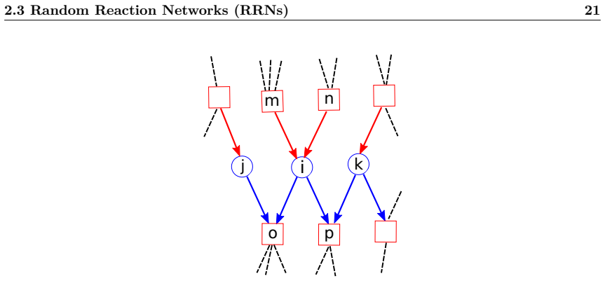
The central object is the pair of constraints of Section 2.1, written compactly in (2.9)-(2.10): $\Gamma_m = \delta_{\mu_m,0}\delta_{x_m,0}(\delta_{y_m,0})^\alpha + \delta_{\mu_m,1}(1-\delta_{x_m,0})(1-\delta_{y_m,0})^\alpha$ and $\Delta_i = \delta_{\nu_i,0} + \delta_{\nu_i,1}\prod_{m\in\partial_i^{\mathrm{in}}}\mu_m$, where $\alpha=1$ gives Hard-MB, $\alpha=0$ gives Soft-MB, $\nu_i\in\{0,1\}$ says whether reaction $i$ runs, $\mu_m\in\{0,1\}$ whether metabolite $m$ is available, and $x_m$, $y_m$ count the active reactions producing and consuming $m$. The argument is carried by casting these constraints as factor nodes of a factor graph and solving the belief-propagation (cavity) equations derived in Section 4.1: population dynamics for ensemble-averaged behaviour, BP plus decimation to generate individual configurations, and a mean-field limit at $\theta\to\infty$ that is shown to coincide with the established Network Expansion procedure. This machinery yields a phase diagram in the topology parameters $(\lambda, q)$ and produces the explicit configuration samples on E. coli from which functional modules are extracted.

What would settle it

Measure real E. coli flux states (for instance by 13C-based flux analysis on glucose minimal medium), convert each measured state into a Boolean pattern of active reactions and available metabolites, and count violations of constraints (2.9)-(2.10)—in particular active reactions whose substrates are not produced by any active reaction, or available metabolites with no active producer (and, under Hard-MB, no active consumer). If a substantial fraction of measured states violates these rules, the Boolean characterization of feasible states fails; if violations are systematically absent, the central claim is supported.

Watch

Extended reading notes

Core claim

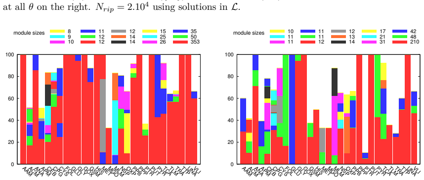
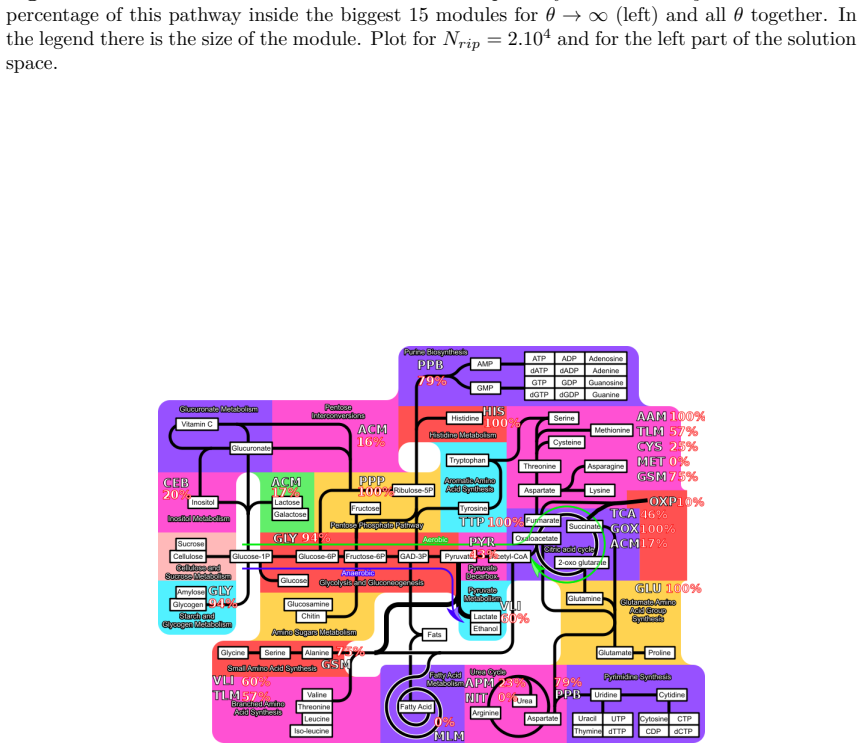
The central claim is that a Boolean description suffices to characterise the feasible non-equilibrium steady states of a reaction network. Two CSPs are defined. In both, a reaction is SAT only if all its input metabolites are available ($\Delta_i = \delta_{\nu_i,0} + \delta_{\nu_i,1} \prod_{m\in\partial_i^{\mathrm{in}}}\mu_m$), and a metabolite is SAT either when it is unavailable and untouched by active reactions, or when it is available and at least one active reaction produces it—with, in the Hard-MB version (constraint (2.9), $\alpha=1$), also at least one active reaction consuming it. A non-trivial assignment of reaction states $\nu_i$ satisfying all reaction and metabolite constraints is declared a feasible operational state. On random reaction networks the paper maps how the solution space changes with topology: Soft-MB sustains solutions across a wide range of activity levels with a region of hysteresis at high connectivity, while Hard-MB shows strong first-order-like hysteresis almost everywhere and essentially forbids sparse states. In preliminary results on the E. coli network, sampling the solutions recovers functional modules—the largest of which is the aerobic respiration pathway set—suggesting that this CSP class is a quantitative link between network structure and metabolic function.

Load-bearing premise

The load-bearing premise is the Boolean modeling rule introduced in Eqs. (2.4)-(2.6): a reaction can run only when all its input metabolites are present, and a metabolite counts as present exactly when at least one active reaction produces it—with the Hard version also demanding an active consumer—so if real metabolic states regularly violate this on/off abstraction, the sampled feasible configurations are not biological states.

Editorial extensions

If this is right

Metabolic feasibility becomes a decision problem solvable from topology alone: for a given network and nutrient availability, an on/off assignment of reactions and metabolites either satisfies constraints (2.9)-(2.10) or not, with no kinetic or thermodynamic parameters required.
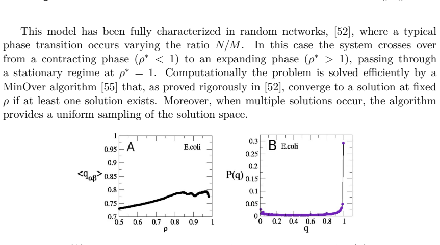
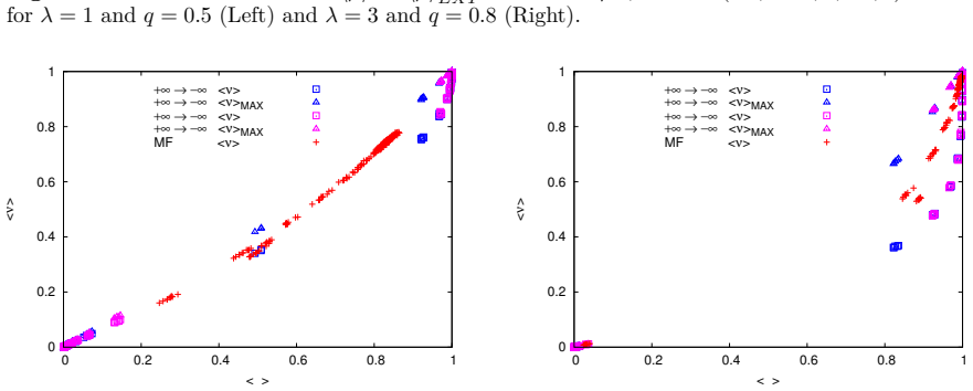
The solution space is structured: on random networks the feasible states display hysteresis and first-order-like transitions, especially under Hard-MB, so a single network can admit qualitatively distinct coexisting operational regimes.
For E. coli, sampling feasible states exposes functional modules—the largest module is the aerobic-respiration pathway set—giving a direct read-off of structure-to-function mapping.
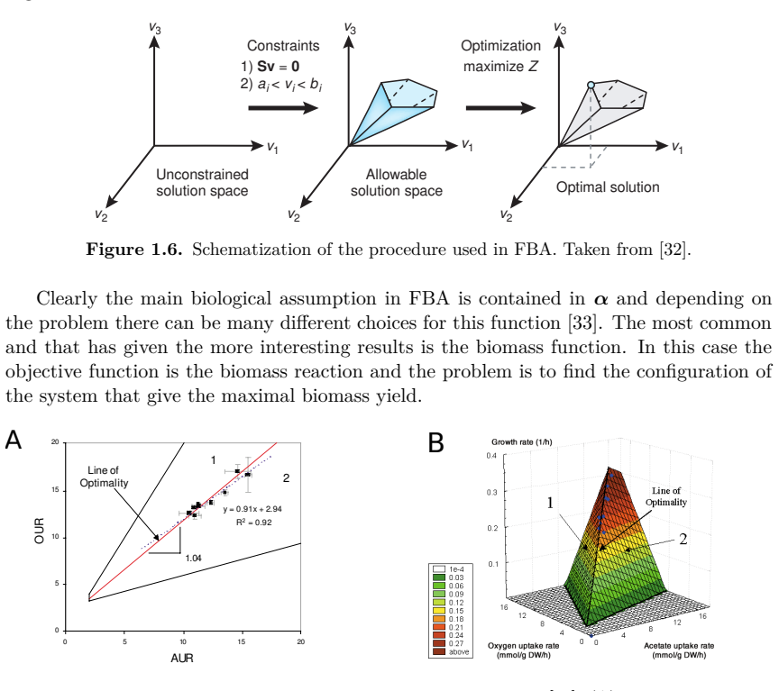
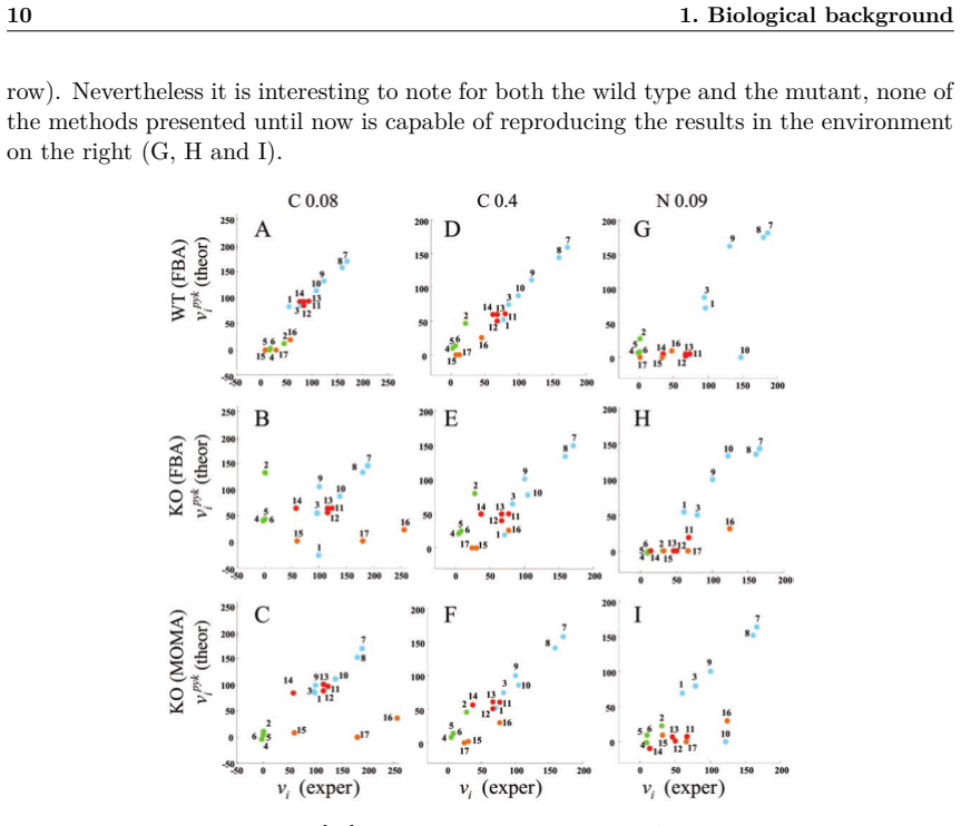
The framework interpolates between known methods: in the mean-field limit it reduces to Network Expansion, and it supplies Boolean counterparts to Flux Balance Analysis and the Von Neumann growth model, while sampling the whole feasible space instead of one optimum.
Topological redundancy is what makes sparse states possible: Boolean solutions with few active reactions exist only for networks with sufficiently large metabolite degree $\lambda$, giving a concrete sense in which redundancy confers flexibility.

Reading between the lines

Editorial extensions of the paper, not claims the author makes directly.

A natural test follows: feed the sampled Boolean configurations into FBA's linear mass-balance constraints and check which ones also admit non-zero real fluxes; the thesis flags this as future work, but it is the direct way to check whether the Boolean feasibility space and the flux feasibility space coincide.
The hysteresis found in random networks suggests a regulation-free source of phenotypic heterogeneity: even with nutrients fixed, the constraints alone admit multiple coexisting activity regimes, which could underpin phenomena like bacterial persistence without invoking gene regulation.
The fraction of reactions frozen at each plateau of the E. coli Hard-MB magnetization could be compared with experimentally known essential genes; a strong overlap would make the model a predictor of minimal gene sets.

Share X Bluesky LinkedIn Reddit HN

Signed reviews

No signed human review yet.

Editorial analysis

A structured set of objections, weighed in public.

Desk editor's note, referee report, and a circularity audit.

Desk Editor's Note

read the letter

Dear [Colleague],

You should know this is a PhD thesis from 2013 posted to arXiv in 2019, not a peer-reviewed paper. That context matters: the random-network part is a genuine methodological contribution, the E. coli part is explicitly preliminary and should not be read as established biology.

What's actually new: two Boolean CSPs, Hard-MB and Soft-MB, that encode mass-balance-like constraints on reaction/metabolite activity; the cavity equations for them; a mean-field limit that recovers network expansion; and a phase diagram for random reaction networks showing hysteresis for Hard-MB and a percolation-type transition for the MF/NE limit. The message-passing equations look internally consistent, and the MF equivalence is a useful formal link. I checked the constraint definitions and the cavity equations: they are coherent.

Where it is soft: the central biological claim is that solutions of these CSPs characterize feasible operational states. The paper itself concedes in Section 4.2 that not every Hard-MB solution can carry non-zero flux in the linear FBA problem, and the count condition M⟨μ⟩≤N⟨ν⟩ is necessary, not sufficient. So the CSPs describe a superset of flux-realizable states. That gap is never closed: no constructive flux assignment, no lifting theorem, no numerical check on the sampled E. coli modules. The Boolean AND/OR abstraction discards concentrations, kinetics, reversibility, and thermodynamics; whether that is a faithful minimal description is argued, not demonstrated. The E. coli module analysis is a pilot: no error bars, no code/data release, Nrip=2×10^4, and module cutoff chosen via a heuristic. For a thesis that's fine; for a published claim it's thin.

Also, it's a thesis, so the exposition is uneven: long background chapters, some equations are dense and not fully derived, and the references are a bit dated. No serious issue with the citation pattern, though.

Bottom line: as a source of new ideas and a formal link between Boolean CSPs and network expansion, it deserves a read and a cite if you work on coarse-grained metabolic models. As evidence about E. coli functional modules, it is not yet referee-ready on its own; it would need code, data, and a flux-realizability check. If you're choosing whether to send it to a journal referee, I would send it—the methodological content justifies a careful review even if the biology needs work.

Referee Report

4 major / 5 minor

Summary. This 2013 PhD thesis, posted on arXiv, introduces two Boolean constraint satisfaction problems, called Hard-MB and Soft-MB, as coarse-grained descriptions of non-equilibrium steady states of reaction networks. Each reaction carries a Boolean variable ν_i and each metabolite a Boolean variable μ_m; the constraints (Eqs. 2.9 and 2.10) require an active reaction to have all its input metabolites available, a metabolite to be available when at least one active reaction produces it (Soft-MB), and, in Hard-MB, additionally to have at least one active consumer. The thesis derives cavity and belief-propagation equations for these CSPs on a random reaction network ensemble, studies the resulting phase diagrams by population dynamics, identifies hysteresis and first-order-like transitions, shows that the θ→∞ mean-field limit reduces to network expansion, and applies the framework to the E. coli K-12 metabolic network, where it clusters reactions into ``functional modules'' using a correlation matrix and a cutoff chosen by an entropy heuristic. The random-network analysis is the main technical contribution; the E. coli results are explicitly presented as preliminary.

Significance. If the claim that Hard-MB and Soft-MB solutions characterize feasible operational states of reaction networks were established, the paper would provide a new structural coarse-graining of metabolism, potentially allowing statistical-physics sampling of suboptimal states that standard FBA cannot easily explore. The paper has real strengths: the mean-field equations for network expansion (Eq. 4.17) are derived analytically and are free of fitted parameters; the population-dynamics, BP, and decimation results agree qualitatively on random networks; and the θ→∞ limit correctly reproduces known network-expansion behavior on E. coli. However, the central biological claim is not yet supported. The manuscript itself concedes that not every Hard-MB solution carries a non-vanishing flux in the linear problem (Section 4.2), and the proposed count condition M⟨μ⟩ ≤ N⟨ν⟩ is only necessary, not sufficient. The E. coli module analysis lacks error bars, convergence diagnostics, and any independent flux validation, and it is performed without reversible reactions.

major comments (4)

[§2.1 and §4.2, especially Eq. (2.9)-(2.10) and Fig. 4.9] The central claim that Hard-MB and Soft-MB solutions describe feasible operational states is not established. The paper itself states in Section 4.2 that ``not all of the solutions to Hard-MB would be able to carry non-vanishing fluxes in the linear problem defined by (2.1)'', and then invokes the comparison M⟨μ⟩ ≤ N⟨ν⟩ as a realizability criterion. That inequality is necessary but not sufficient: a Boolean pattern can satisfy it while no positive flux vector J with J_i > 0 on the active support and J_i = 0 on the inactive support solves S_active J = 0 (or S_active J ≥ 0 for Soft-MB). No lifting theorem, constructive flux assignment, or numerical FBA validation is provided. Consequently the CSPs currently characterize a superset of FBA/Von Neumann states, not the feasible states themselves, and the biological reading of the E. coli modules inherits this gap.
[§5.1, §5.3.2, and §5.4] The E. coli functional-module analysis is not validated against flux or growth data. Section 5.1 promises that sampled configurations will be checked with FBA, but no such FBA check is reported. The modules are obtained by correlating Boolean solutions that are restricted by ad hoc axioms (7 nutrients ON, ATPM active, single connected component) and by a cutoff C~ chosen through the heuristic H(C~) versus H({n_i}) criterion (Eqs. 5.6-5.7). No error bars, sampling repeatability statistics, convergence diagnostics, or code/data are provided. The observation that the recovered modules overlap known biochemical pathways is suggestive, but it does not establish that these Boolean patterns are realizable metabolic states; a direct FBA-flux validation on the sampled configurations would be needed.
[§5.2-§5.4 and Chapter 6] Reversibility, which the text identifies as a key feature of E. coli (about 40% of reactions), is not included in any reported result. Section 5.2 derives the reversible constraint Ω(ν_i, ν_{-i}) = 1 - ν_i ν_{-i}, but Section 5.4 presents only the ``non reversible case'', and the Conclusions explicitly list ``develop the reversible BP and decimation algorithm'' as future work. The module analysis in Section 5.3.2 is performed under the mean-field approximation, where the text says the reversibility constraint cannot be added. Since ignoring reversibility can change which steady states exist, the E. coli results cannot be read as an analysis of the actual metabolic network.
[§2.1, Eqs. (2.4)-(2.6)] The Boolean abstraction discards stoichiometric coefficients, concentrations, kinetics, reversibility, and thermodynamics, yet the paper does not test its faithfulness as a minimal description of metabolic steady states. The claim that the CSPs ``describe the feasible operational states'' would require at least a numerical comparison of Hard-MB/Soft-MB predicted active/inactive patterns against FBA solutions or 13C flux data on the same E. coli network. Absent such a check, the Boolean rule is an assumption rather than a demonstrated characterization, and this is a load-bearing limitation for the paper's central claim.

minor comments (5)

[§1.2, Eq. (1.7)] The displayed formula for the Euclidean distance in MOMA is garbled; the radical and summation are illegible. This should be typeset cleanly.
[§3.1, Eq. (3.1)] The soft-CSP weight ψ_a^β = e^{-β(1-ψ_a(σ_∂a))} appears dimensionally inconsistent with the stated Hamiltonian H = Σ_a (1-ψ_a(σ_∂a)); presumably the intended weight is e^{-β H_a}. Please reconcile the notation.
[Throughout, especially §4.1 and §4.2] The symbol α is used for multiple purposes: the interpolation parameter between Soft-MB and Hard-MB, the FBA objective coefficients in Chapter 1, and implicitly elsewhere. Renaming one of these would improve readability.
[§2.2 and Table 2.1] The E. coli network description gives no version of the stoichiometric model, no reaction count, and no source for the network reconstruction beyond citing iJR904; the biomass table also lacks explicit units. This makes the E. coli results hard to reproduce.
[§5.3.2, Figs. 5.4-5.7] The module-size histograms and the H(C~) curves are presented without error bars or sensitivity analysis with respect to the cutoff; adding a stability analysis of the modules under perturbations of C~ would make the clustering result more convincing.

Circularity Check

0 steps flagged · score 0.0 of 10

No circularity: the CSPs are analyzed from their explicit definitions and compared against external benchmarks.

full rationale

The paper derives the Hard-MB and Soft-MB CSPs directly from the linear mass-balance conditions (2.1) and (2.2), stating the constraints in Eqs. (2.4)-(2.10) rather than importing them from a fitted model. The later results (phase diagrams, hysteresis, E. coli modules) are obtained by running population dynamics, BP, and decimation on those definitions while sweeping the control parameters θ and ρ_in; no parameter is fitted to reproduce the reported phase behavior or module structure. The mean-field limit is shown to coincide with Network Expansion via a derivation (Section 4.3), and the E. coli modules are validated against known biochemical pathways, which is an external comparison rather than an input. Self-citations to the advisors' earlier Von Neumann papers occur in background sections and are not load-bearing for the new CSP derivation. The admitted limitation that some Hard-MB solutions cannot carry non-vanishing FBA fluxes (Section 4.2.2) is a correctness caveat, not a circular step, since the paper does not redefine realizability to make the claim true by construction.

Assumptions & free parameters 6 free parameters · 5 assumptions · 0 invented entities

The central claim rests on a coarse-grained Boolean model with several hand-set control and sampling parameters. No physical entities are invented. The axioms are a mix of standard statistical mechanics assumptions and biological modeling postulates.

free parameters (6)

θ (chemical potential) = varied continuously from -∞ to +∞ in sweeps
Controls the bias toward active reactions in the measure (4.3); not fitted to data, but the phase diagrams and hysteresis loops are defined in terms of sweeps in θ.
ρ_in (nutrient availability probability) = 0, 0.5, 1 and intermediate values
Boundary probability that a nutrient is initially available; varied to test environment effects in Figures 4.3-4.7.
λ (mean metabolite degree) = 1 to 3.5 in phase maps
Poisson mean of in/out degrees for metabolite nodes in the RRN ensemble; a parameter of the random graph model, not fitted to data.
q (reaction degree mixing) = 0 to 1
Probability that a reaction has degree 2 instead of 1; a parameter of the RRN ensemble.
p (initial internal activation probability in E. coli sampling) = 0 to 0.1
In Section 5.3.2, internal metabolites are initialized active with small probability p while nutrients are fixed ON; this restriction is a hand-set sampling bias.
module cutoff C~ = chosen at entropy maximum
Correlation-matrix cutoff used to convert the correlation graph to an adjacency matrix and define modules; this choice affects all module results in Section 5.3.2.

assumptions (5)

domain assumption A reaction network state can be coarse-grained to binary variables ν_i and μ_m with constraints (2.9)-(2.10) capturing operational feasibility.
The entire CSP definition is a modeling postulate introduced in Section 2.1; the paper calls the constraints 'minimal necessary requirements', not proven equivalents of FBA or VN.
domain assumption A reaction is active only if all its input metabolites are available (Eqs. 2.6 and 2.10).
Used to define Δ_i; this AND-like rule ignores concentration levels, kinetics, and thermodynamics.
standard math Cavity and Bethe equations assume locally tree-like graphs and decorrelated incoming messages.
Valid for random networks with loops of length log N, but not guaranteed for the E. coli network, which the text acknowledges has many short loops (Section 5.1).
standard math Mean-field approximation factorizes joint distributions as in Eqs. (4.9)-(4.10).
Used to derive the PEI equations (4.5)-(4.6) and the phase diagram (4.17); ignores correlations among reaction and metabolite variables.
ad hoc to paper In the E. coli analysis, solutions are restricted to those with 7 nutrients ON, ATPM active and a single connected component.
Introduced in Section 5.1 to restrict the huge solution space; not derived from data or first principles.

how reviews work

0 comments

Cite this review

Pith. "Pith review of Boolean constraint satisfaction problems for reaction networks." pith.science (2026). https://pith.science/paper/HBVMCKU2

@misc{pith2026190804836,
  author       = {Pith},
  title        = {Pith review of: Boolean constraint satisfaction problems for reaction networks},
  year         = {2026},
  howpublished = {\url{https://pith.science/paper/HBVMCKU2}},
  note         = {Machine review of arXiv:1908.04836}
}

read the original abstract

This Thesis presents research at the boundary between Statistical Physics and Biology. First, we have devised a class of Boolean constraint satisfaction problems (CSP) whose solutions describe the feasible operational states of a chemical reaction network. After developing statistical mechanics techniques to generate solutions and studying the properties of the solution space for both ensembles and individual instances of random reaction networks, we have applied this framework to the metabolic network of the bacterium E.Coli. Results highlight, on one hand, a complex organization of operational states into "modules" involving different biochemically-defined pathways, and, on the other, a high degree of cross-talk between modules. In summary, we propose that this class of CSPs may provide novel and useful quantitative information linking structure to function in cellular reaction networks.

Figures

Figures reproduced from arXiv: 1908.04836 by the authors.

**Figure 1.1.** Schematic representation of the Metabolism divided in pathways. In each square there is the pathway name and the key metabolites involved in this pathway. [21] In this section we will briefly summarize the most important characteristics of metabolism, for a comprehensive approach of this argument see [22]. Metabolism is the combination of processes through which cells make and use the energy needed for all their phy… view at source ↗

**Figure 1.2.** Schematic representation of the Glycolysis. parts of the cell producing substrates needed by the cell. The main catabolic pathways are: the Glycolysis and the Krebs cycle (or TCA cycle) that we will detail further in the following. Whereas anabolic pathways can be divided in four main groups: the fatty acid metabolism, for the synthesis of the elements of the membrane of the cell, the nucleotide synthesis pathways,… view at source ↗

**Figure 1.3.** Schematic representation of the Krebs cycle. Glycolysis is the pathway by which the cell decomposes glucose in smaller molecules. The net energy yield of this pathway are two molecules of ATP per molecule of glucose as it uses two ATP molecules and produces four, see [PITH_FULL_IMAGE:figures/full_fig_p010_1_3.png] view at source ↗

Figures from the paper (57 more)

**Figure 1.4.** Figure 1.4: Typical bacterial growth in a suitable environment. [23] energetic point of view than fermentation. The combination of Glycolysis and Krebs Cycle is called aerobic respiration. This is clearly the most efficient process to produce energy and it is the preferred pathw…

**Figure 1.5.** Figure 1.5: Sketch of a bipartite network representing a metabolic network, where the squares are the metabolites and the circles the reactions. is then possible, by measuring the final products of the cell, to reconstruct from which pathways the glucose has been processed. Neve…

**Figure 1.6.** Figure 1.6: v2 v1 v3 Allowable solution space Optimal solution v3 Unconstrained solution space Constraints 1) Sv = 0 2) ai < vi < bi v2 v2 v1 v3 Optimization maximize Z v1 [PITH_FULL_IMAGE:figures/full_fig_p014_1_6.png]

**Figure 1.7.** Figure 1.7: Predictions and experimental results obtained in article [34]. (A) acetate uptake rate (AUR, mmol/g DW/h) versus oxygen uptake rate (OUR, mmol/g DW/h). The red line is the LO and the points are the experimental measurement. (B) 3D representation of the same results. …

**Figure 1.8.** Figure 1.8: Results obtained in article [37]. (A-C) glycerol uptake rate (Gl-UR) versus oxygen uptake rate (OUR) in a colony of E.Coli starting from day 0 to day 60. LO is the line of optimality and the dots and crosses are the experimental results. In [37] the authors used the …

**Figure 1.9.** Figure 1.9: Schematic of the MOMA method developed in [38]. In [38] the authors extended FBA to deal with the mutations and knock outs of genes, developing a quadratic programming method named minimization of metabolic adjustment (MOMA). In this method, if a mutation occurs, the…

**Figure 1.10.** Figure 1.10: Results of article [38]. The column correspond to different environment conditions. In each graph the measured fluxes of reactions from the central carbon metabolism are plotted versus the computed fluxes. The first row represents the FBA results for the Wild Type E…

**Figure 1.11.** Figure 1.11: After establishing the predictive power of FBA, this model was used to predict the capabilities and properties of real networks for various organisms. The robustness of the network to the deletion of chosen reactions was analyzed in [41] using a method called Flux V…

**Figure 1.12.** Figure 1.12: Comparison of the value of the fluxes between theoretical values obtain by VN and experimental points (in red). ([53]) metabolites 100 200 300 400 500 600 100 200 300 400 500 0 2 4 6 8 10 12 [PITH_FULL_IMAGE:figures/full_fig_p019_1_12.png]

**Figure 1.13.** Figure 1.13: Values of c m for different metabolites in 500 different solutions ([53]). This model has been fully characterized in random networks, [52], where a typical phase transition occurs varying the ratio N/M. In this case the system crosses over from a contracting phase …

**Figure 1.14.** Figure 1.14: (A) Mean overlap in 500 solutions of VN versus the value of ρ. (B) Distribution of the q (i) αβ overlap. ([53]). In [53] this method was applied to the metabolic network of E.Coli as the metabolism of a real network can still be modeled as an autocatalytic system if…

**Figure 1.15.** Figure 1.15: Sketch of four steps of NE procedure in an idealized metabolic network. The metabolites contained in the seed are in black. growing. It is though possible to define the set of sustainable metabolites (S(U)) which are the ones that the cell will continue to produce a…

**Figure 2.1.** Figure 2.1: In- and out-degrees of E.Coli for metabolites and reactions. E.Coli is generally considered a model organism as it is inexpensive to grow in laboratory due to its little generation rate and to the fact that the K-12 strain is easily cultivated. Furthermore its metab…

**Figure 2.2.** Figure 2.2: Sketch of a random reaction network of the type discussed in the text. m, n, o and p denote metabolites (squares), i, j and k are instead reactions (circles). Red (resp. blue) links carry substrate-like (resp. product-like) couplings with ξ m i = −1 (resp. ξ p i = 1)…

**Figure 2.3.** Figure 2.3: Sketch of the factor graph representation of a RRN. Here squares represent metabolite variables, circles reaction variables, hexagons metabolite-constraints and triangles reactionconstraints. or N = λM/(1 + q). In order to compute the equations for the system it is…

**Figure 3.1.** Figure 3.1: Sketch of the factor graph representation of a CSP. 23 [PITH_FULL_IMAGE:figures/full_fig_p029_3_1.png]

**Figure 3.2.** Figure 3.2: Plot of the r.h.s. and l.h.s. of equation (3.5) for various values of λ. that is a Poissonian distribution. This type of distribution has the characteristic that the probability of having a vertex with degree d λ decreases exponentially. In random graphs typical loop…

**Figure 3.3.** Figure 3.3: Representation of a GN,6 cavity graph on a lattice with k = 2. Hence q = 6 spins have 2 neighbours and all other N − 6 remaining spins have 3 neighbours (taken from [79]). It is instructive to compute the free energy at zero temperature on a Bethe lattice with fixed …

**Figure 3.4.** Figure 3.4: Sketch of the 1-d Ising model under consideration • (site addition) add a new spin σ0, connect it to k+1 cavity spins and then optimizing the values of the k + 2 spins; in this case we are transforming a GN,q graph to a GN+1,q−k−1 graph (δN = 1 and δq = −k − 1). Thus…

**Figure 3.5.** Figure 3.5: Sketch of the messages sent in part of a factor graph. In this situation, the Bethe Approximation consist in considering that the messages arriving from vertices a and b are not correlated although it is clear that this is not true. is straightforward to write the Gi…

**Figure 3.6.** Figure 3.6: Sketch of the cavity messages in a factor graph In cases in which it is not possible to make the simplification of removing the factor node (see [PITH_FULL_IMAGE:figures/full_fig_p038_3_6.png]

**Figure 3.7.** Figure 3.7: Sketch of the set of solutions in the q-col problem as the average connectivity, c, changes. Black clusters have all variables frozen while grey clusters no (taken from [101]). find the equations also in this part of the phase space. Following this ideas, the authors…

**Figure 4.1.** Figure 4.1: Summary of the cavity method messages for Soft-MB (left) and Hard-MB (right) constraints [PITH_FULL_IMAGE:figures/full_fig_p044_4_1.png]

**Figure 4.2.** Figure 4.2: Soft-MB: behaviour of the average fraction of available metabolites, hµi (left) and of the average fraction of active reactions, hνi (right) versus θ for different values of the parameters λ and q and fixed ρin = 0.5. defined by q and λ, by the fact that a certain se…

**Figure 4.3.** Figure 4.3: Map of the values of ∆µ (normalized by the same maximum: 4.852) for the Soft-MB problem in the (λ, q) plane. The spacing in q is equal to 0.01, while it is 0.1 in λ. A) ρin = 0; B) ρin = 1. average metabolite availability seems to concentrate in small ranges close to…

**Figure 4.4.** Figure 4.4: Map of the values of ∆µ (normalized by the same maximum: 12.643) for the HardMB problem in the (λ, q) plane. The spacing in q is equal to 0.01, while it is 0.1 in λ. A) ρin = 0; B) ρin = 1. 0 0.2 0.4 0.6 0.8 1 -4 -2 0 2 4 < —ν > θ λ=1, q =0.8 S-MB +∞ → −∞ S-MB −∞ → …

**Figure 4.5.** Figure 4.5: Behaviour of hµi+ and hµi− (left) and hνi+ and hνi− (right) as functions of θ at λ = 1, q = 0.8 and ρin = 0.5 for the Soft- and Hard-MB problems. 0 0.2 0.4 0.6 0.8 1 -4 -2 0 2 4 < —ν > θ λ=3, q =0.9 S-MB +∞ → −∞ S-MB −∞ → +∞ H-MB +∞ → −∞ H-MB −∞ → +∞ 0 0.2 0.4 0.6 0.…

**Figure 4.6.** Figure 4.6: Behaviour of hµi+ and hµi− (left) and hνi+ and hνi− (right) as functions of θ at λ = 3, q = 0.9 and ρin = 0.5 for the Soft- and Hard-MB problems [PITH_FULL_IMAGE:figures/full_fig_p049_4_6.png]

**Figure 4.7.** Figure 4.7: Spinodal values for the existence of upper and lower branches of hµi (θ+ and θ−, respectively) for Soft-MB and Hard-MB. Left panel: ρin = 0; Right panel: ρin = 1. 0 0.2 0.4 0.6 0.8 1 0 0.2 0.4 0.6 0.8 1 P(<—>) i < —i > Soft-MB LOW Soft-MB HIGH Hard-MB LOW Hard-MB HIG…

**Figure 4.8.** Figure 4.8: Histogram of the values of the average availability of metabolites (left) and reactions (right) for λ = 3, q = 0.8 and ρin = 0.5. The value of θ has been chosen for both CSPs at the transition, so that both high and low values of hµi and hνi are possible. In specific…

**Figure 4.9.** Figure 4.9: Left: behaviour of hµi versus N M hνi (left) and versus hνi (right) for λ and q as displayed in the legend. In each dataset θ increases from left to right. From the distribution of metabolite availabilities one clearly sees that, generically, fluctuations are larger …

**Figure 4.10.** Figure 4.10: Sketch of four steps of the Propagation of External Inputs (PEI) algorithm (serving as the basis of the Network Expansion method [18]). Black squares represent compounds initially available. In step 1, reaction i is activated by virtue of the availability of compoun…

**Figure 4.11.** Figure 4.11: Phase diagram obtained by propagation of external inputs (PEI) in the (q, λ) plane. The insets display the curves γ versus ρin obtained in the different sectors; all lines are analytical. See text for details. For any fixed ρin, whenever solutions with different val…

**Figure 4.** Figure 4: ) are, in essence, of a percolation type. [PITH_FULL_IMAGE:figures/full_fig_p054_4.png]

**Figure 4.12.** Figure 4.12: Theoretical solution of Equation (4.17) (solid line) versus ρin, together with the results obatined by PEI and reverse-PEI. 0 0.2 0.4 0.6 0.8 1 0 0.2 0.4 0.6 0.8 1 γ ρin γmax=1-γ0 γ1 γ0 γPER 0 0.2 0.4 0.6 0.8 1 0 0.2 0.4 0.6 0.8 1 γ ρin [PITH_FULL_IMAGE:figures/ful…

**Figure 4.13.** Figure 4.13: Weights of the different components of the PER core for a graph with λ = 3 and q = 0.87. The red line corresponds to the solution of equation (4.17) [PITH_FULL_IMAGE:figures/full_fig_p055_4_13.png]

**Figure 4.14.** Figure 4.14: Graph of all the component of the PER core for a graph with λ = 3 and q = 0.87. The red line is the solution of equation (4.17). In turn, one obtains τ0 = 1 − q(1 − γ0) 2 − (1 − q)(1 − γ0) , (4.22) γ0 = e −λ e λτ0 − ρine −λ , (4.23) τ1 = qγ2 1 + (1 − q)γ1 , (4.24) γ…

**Figure 4.15.** Figure 4.15: Soft-MB for λ = 1, q = 0.5 and ρin = 1. Left: average fraction of available metabolites, hµi (hµi for population dynamics) versus θ. Right: average fraction of active reactions, hνi (hνi for population dynamics) versus θ. 0 0.2 0.4 0.6 0.8 1 -4 -2 0 2 4 —< >,< > θ …

**Figure 4.16.** Figure 4.16: Soft-MB for λ = 3, q = 0.8 and ρin = 1. Left: average fraction of available metabolites, hµi (hµi for population dynamics) versus θ. Right: average fraction of active reactions, hνi (hνi for population dynamics) versus θ. Results are presented in Figures 4.15 and 4…

**Figure 4.17.** Figure 4.17: Hard-MB for λ = 1, q = 0.5 and ρin = 1. Left: average fraction of available metabolites, hµi (hµi for population dynamics) versus θ. Right: average fraction of active reactions, hνi (hνi for population dynamics) versus θ. 0 0.2 0.4 0.6 0.8 1 -4 -2 0 2 4 —< >,< > θ …

**Figure 4.18.** Figure 4.18: Hard-MB for λ = 3, q = 0.8 and ρin = 1. Left: average fraction of available metabolites, hµi (hµi for population dynamics) versus θ. Right: average fraction of active reactions, hνi (hνi for population dynamics) versus θ. 0 0.2 0.4 0.6 0.8 1 -4 -2 0 2 4 —< >,< > θ …

**Figure 4.19.** Figure 4.19: Soft-MB: behaviour of the average fraction of available metabolites, hµi (hµi for population dynamics) for λ = 1 and q = 0.5 (Left) and λ = 3 and q = 0.8 (Right) at various ρin [PITH_FULL_IMAGE:figures/full_fig_p058_4_19.png]

**Figure 4.20.** Figure 4.20: Soft-MB: Plot of hµi vs hµiEXT for various ρin, for θ = (−5, −4.5, .., 4.5, 5) and for λ = 1 and q = 0.5 (Left) and λ = 3 and q = 0.8 (Right). 0 0.2 0.4 0.6 0.8 1 0 0.2 0.4 0.6 0.8 1 < ν > < > +∞ → −∞ <ν> +∞ → −∞ <ν>MAX +∞ → −∞ <ν> +∞ → −∞ <ν>MAX MF <ν> 0 0.2 0.4 0.…

**Figure 4.21.** Figure 4.21: Plot of hµi versus hνi for λ = 1 and q = 0.5 (Left) and λ = 3 and q = 0.8 (Right). between the average magnetization of reactions and metabolites and both ρin and hµiEXT in Figures 4.19 and 4.20. We first note that in this way we are able to obtain solutions at vari…

**Figure 5.1.** Figure 5.1: Scope of the seed versus θ. The points are after the decimation process, while the lines are given only by the BP procedure 5.3 Mean Field Approximation As we already explained the MF case for θ → ∞ is a different formulation of a better known problem called Network …

**Figure 5.2.** Figure 5.2: Scope Σ(U) of the seed U in the region between p = [0, 0.1] for θ → ∞ with one connected component and 7 nutrients ON, here Nrip = 104 . 0 0.002 0.004 0.006 0.008 0.01 0 100 200 300 400 500 600 700 800 freq REA ON θ=0.5 θ=1 θ=1.5 θ=2 θ=2.5 θ→ ∞ 0 0.002 0.004 0.006 0.…

**Figure 5.3.** Figure 5.3: Histogram of the number of reactions functioning in the region between p = [0, 0.1] for some θ on the left and the cumulative plot for all θ on the right. All solutions have one connected component and 7 nutrients ON, here Nrip = 2.104 . The protocol that we will use…

**Figure 5.** Figure 5: , that is the cumulative histogram over all [PITH_FULL_IMAGE:figures/full_fig_p064_5.png]

**Figure 5.4.** Figure 5.4: H(C˜) in function of H({ni}) for both θ → ∞ (left) and for the cumulative solutions at all θ on the right. Nrip = 2.104 using solutions in R. In the following we will focus on the reactions as they have already been divided in pathways (see Chapter 1) thus it will be…

**Figure 5.5.** Figure 5.5: H(C˜) in function of H({ni}) for both θ → ∞ (left) and for the cumulative solutions at all θ on the right. Nrip = 2.104 using solutions in L. 0 20 40 60 80 100 AAM ACM ANAAPMCEB CPG CYSFOLGLU GLYGOX GSMHIS MET MGO MLM NSPOXP PPBPPPPTR PUTPYR TCATLM TRA TTPUNA VLI mod…

**Figure 5.6.** Figure 5.6: On the x axis there is the name of the pathway while on the y axis there is the percentage of this pathway inside the biggest 15 modules for θ → ∞ (left) and all θ together. In the legend there is the size of the module. This plot is for Nrip = 2.104 and for the righ…

**Figure 5.7.** Figure 5.7: On the x axis there is the name of the pathway while on the y axis there is the percentage of this pathway inside the biggest 15 modules for θ → ∞ (left) and all θ together. In the legend there is the size of the module. Plot for Nrip = 2.104 and for the left part of…

**Figure 5.8.** Figure 5.8: Representation of the modules we find divided in pathways for the right part of the solutions. The numbers below the pathways are the percentage of reactions of the pathway switched on. The cutoff is at 0.983 [PITH_FULL_IMAGE:figures/full_fig_p067_5_8.png]

**Figure 5.9.** Figure 5.9: Soft-MB solutions for the reactions (right) and the metabolites (left) in the irreversible case. Solutions are found using the BP algorithm (BP) and the decimation (DEC) algorithm for various θ. Here we present only the results for the protocol +∞ → −∞ because the ot…

**Figure 5.10.** Figure 5.10: Hard-MB solutions for the reactions (right) and the metabolites (left) in the irreversible case. Solutions are found using the BP algorithm (BP) and the decimation algorithm for various θ. is dependent on how many solutions are sampled in this part. It is also inte…

**Figure 5.11.** Figure 5.11: Marginal of the reactions in Hard-MB, for the case +∞ → ∞ and ρin = 1. to verify which solution is using which nutrient, to understand the organization of the solution space (work in progress). It is thus clear from these results that exactly as we found on the rand…

Discussion (0). Continue with ORCID to comment.

Reference graph

Works this paper leans on

110 extracted references · 79 canonical work pages

[1]

Network biology: understanding the cell’s functional organization

A-L Barabási and Z N Oltvai. Network biology: understanding the cell’s functional organization. Nature Reviews Genetics, 5(2):101, 2004

2004
[2]

Cell biology: Networks, regulation, pathways.Encyclopedia of Complexity and Systems Science, pages 719–741, 2009

G Tkacik and W Bialek. Cell biology: Networks, regulation, pathways.Encyclopedia of Complexity and Systems Science, pages 719–741, 2009

2009
[3]

Kegg for integra- tion and interpretation of large-scale molecular data sets.Nucleic acids research, 40(D1):D109–D114, 2012

M Kanehisa, S Goto, Y Sato, M Furumichi, and M Tanabe. Kegg for integra- tion and interpretation of large-scale molecular data sets.Nucleic acids research, 40(D1):D109–D114, 2012

2012
[4]

The large-scale organization of metabolic networks.Nature, 407(6804):651–654, 2000

H Jeong, B Tombor, R Albert, Z N Oltvai, and A-L Barabási. The large-scale organization of metabolic networks.Nature, 407(6804):651–654, 2000

2000
[5]

Metabolic modelling of microbes: the ﬂux-balance approach.Environmental Microbiology, 4(3):133–140, 2002

J S Edwards, M Covert, and B O Palsson. Metabolic modelling of microbes: the ﬂux-balance approach.Environmental Microbiology, 4(3):133–140, 2002

2002
[6]

Network motifs: Simple building blocks of complex networks

R Milo, S Shen-Orr, S Itzkovitz, N Kashtan, D Chklovskii, and U Alon. Network motifs: Simple building blocks of complex networks. Science, 298(5594):824–827, 2002

2002
[7]

Evolution of evolvability in gene regulatory networks

A Crombach and P Hogeweg. Evolution of evolvability in gene regulatory networks. PLoS computational biology, 4(7), 2008

2008
[8]

Optimality principles in the regulation of metabolic networks.Metabolites, 2(3):529–552, 2012

J Berkhout, F J Bruggeman, and B Teusink. Optimality principles in the regulation of metabolic networks.Metabolites, 2(3):529–552, 2012

2012

Show all 110 references

[9]

Robustness and evolvability: a paradox resolved

A Wagner. Robustness and evolvability: a paradox resolved. Proceedings of the Royal Society B: Biological Sciences, 275(1630):91–100, 2008

2008
[10]

Princeton University Press Princeton, 2005

A Wagner.Robustness and evolvability in living systems. Princeton University Press Princeton, 2005

2005
[11]

Robustness can evolve gradually in complex regulatory gene networks with varying topology.PLoS Computational Biology, 3(2), 2007

S Ciliberti, O C Martin, and A Wagner. Robustness can evolve gradually in complex regulatory gene networks with varying topology.PLoS Computational Biology, 3(2), 2007

2007
[12]

Kauﬀman.The origins of order

S.A. Kauﬀman.The origins of order. Oxford University Press, 1993

1993
[13]

The computational core and ﬁxed point organization in boolean networks.Journal of Statistical Mechanics: Theory and Experiment, 2006(03):P03002, 2006

L Correale, M Leone, A Pagnani, M Weigt, and R Zecchina. The computational core and ﬁxed point organization in boolean networks.Journal of Statistical Mechanics: Theory and Experiment, 2006(03):P03002, 2006

2006
[14]

Motifs emerge from function in model gene regulatory networks.Procedings of the National Academy of Sciences, 108(42):17263–17268, 2011

Z Burda, A Krzywicki, OC Martin, and M Zagorski. Motifs emerge from function in model gene regulatory networks.Procedings of the National Academy of Sciences, 108(42):17263–17268, 2011

2011
[15]

Distribution of essential interac- tions in model gene regulatory networks under mutation-selection balance.Physical Review E, 82(1):011908, 2010

Z Burda, A Krzywicki, OC Martin, and M Zagorski. Distribution of essential interac- tions in model gene regulatory networks under mutation-selection balance.Physical Review E, 82(1):011908, 2010. 71 72 Bibliography

2010
[16]

Design of genetic networks with speciﬁed functions by evolution in silico

P Francois and V Hakim. Design of genetic networks with speciﬁed functions by evolution in silico. Proceedings of the National Academy of Sciences of the United States of America, 101(2):580–585, 2004

2004
[17]

The regulatory network of e

A Samal and S Jain. The regulatory network of e. coli metabolism as a boolean dy- namical system exhibits both homeostasis and ﬂexibility of response.BMC systems biology, 2(1):21, 2008

2008
[18]

Expanding metabolic networks: scopes of compounds, robustness, and evolution

T Handorf, O Ebenhöh, and R Heinrich. Expanding metabolic networks: scopes of compounds, robustness, and evolution. Journal of molecular evolution, 61(4):498– 512, 2005

2005
[19]

Metapath online: a web server implementation of the network expansion algorithm.Nucleic acids research, 35, 2007

T Handorf and O Ebenhöh. Metapath online: a web server implementation of the network expansion algorithm.Nucleic acids research, 35, 2007

2007
[20]

Structural analysis of expanding metabolic networks

O Ebenhöh, T Handorf, and R Heinrich. Structural analysis of expanding metabolic networks. Genome informatics series, pages 35–45, 2004

2004
[21]

Source: http://en.wikipedia.org/wiki/File:Metabolism_790px.png
[22]

T D Brock, M T Madigan, J M Martinko, and J Parker.Brock biology of microor- ganisms 13th ed.Prentice Hall, 2012

2012
[23]

Source: http://en.wikipedia.org/wiki/File:Bacterial_growth_en.svg
[24]

Metabolic networks in motion: 13c-based ﬂux analysis.Molecular systems biology, 2(1), 2006

U Sauer. Metabolic networks in motion: 13c-based ﬂux analysis.Molecular systems biology, 2(1), 2006

2006
[25]

13 c metabolic ﬂux analysis: optimal design of isotopic labeling experiments

M R Antoniewicz. 13 c metabolic ﬂux analysis: optimal design of isotopic labeling experiments. Current Opinion in Biotechnology, 24:1–6, 2013

2013
[26]

Metabolic capabilities of< i> escherichia coli</i> ii

A Varma and B O Palsson. Metabolic capabilities of< i> escherichia coli</i> ii. optimal growth patterns.Journal of Theoretical Biology, 165(4):503–522, 1993

1993
[27]

Monte carlo sampling can be used to determine the size and shape of the steady-state ﬂux space.Journal of theoretical biology, 228(4):437–447, 2004

S J Wiback, I Famili, H J Greenberg, and B O Palsson. Monte carlo sampling can be used to determine the size and shape of the steady-state ﬂux space.Journal of theoretical biology, 228(4):437–447, 2004

2004
[28]

Theory for the systemic deﬁnition of metabolic pathways and their use in interpreting metabolic function from a pathway- oriented perspective

C H Schilling, D Letscher, and B O Palsson. Theory for the systemic deﬁnition of metabolic pathways and their use in interpreting metabolic function from a pathway- oriented perspective. Journal of Theoretical Biology, 203(3), 2000

2000
[29]

N. D. Price, Jennifer L. Reed, Jason A. Papin, Sharon J. Wiback, and B. O. Palsson. Network-based analysis of metabolic regulation in the human red blood cell.Journal of Theoretical Biology, 225, 2003

2003
[30]

On elementary ﬂux modes in biochemical reaction sys- tems at steady state.Journal of Biological Systems, 2(02):165–182, 1994

S Schuster and C Hilgetag. On elementary ﬂux modes in biochemical reaction sys- tems at steady state.Journal of Biological Systems, 2(02):165–182, 1994

1994
[31]

Detection of elementary ﬂux modes in bio- chemical networks: a promising tool for pathway analysis and metabolic engineering

S Schuster, T Dandekar, and D A Fell. Detection of elementary ﬂux modes in bio- chemical networks: a promising tool for pathway analysis and metabolic engineering. Trends in biotechnology, 17(2):53–60, 1999

1999
[32]

What is ﬂux balance analysis? Nature biotechnology, 28(3):245–248, 2010

J D Orth, I Thiele, and B O Palsson. What is ﬂux balance analysis? Nature biotechnology, 28(3):245–248, 2010

2010
[33]

Systematic evaluation of objective functions for predicting intracellular ﬂuxes in escherichia coli.Molecular systems biology, 3(1), 2007

R Schuetz, L Kuepfer, and U Sauer. Systematic evaluation of objective functions for predicting intracellular ﬂuxes in escherichia coli.Molecular systems biology, 3(1), 2007. Bibliography 73

2007
[34]

In silico predictions of escherichia coli metabolic capabilities are consistent with experimental data.Nature biotechnology, 19(2):125–130, 2001

J S Edwards, R U Ibarra, and B O Palsson. In silico predictions of escherichia coli metabolic capabilities are consistent with experimental data.Nature biotechnology, 19(2):125–130, 2001

2001
[35]

Stoichiometric ﬂux balance models quantitatively pre- dict growth and metabolic by-product secretion in wild-type escherichia coli w3110

A Varma and B O Palsson. Stoichiometric ﬂux balance models quantitatively pre- dict growth and metabolic by-product secretion in wild-type escherichia coli w3110. Applied and environmental microbiology, 60(10):3724–3731, 1994
[36]

The escherichia coli mg1655 in silico metabolic genotype: its deﬁnition, characteristics, and capabilities.Proceedings of the National Academy of Sciences, 97(10):5528–5533, 2000

JS Edwards and B O Palsson. The escherichia coli mg1655 in silico metabolic genotype: its deﬁnition, characteristics, and capabilities.Proceedings of the National Academy of Sciences, 97(10):5528–5533, 2000

2000
[37]

Escherichia coli k-12 undergoes adaptive evolution to achieve in silico predicted optimal growth.Nature, 420(6912):186–189, 2002

R U Ibarra, J S Edwards, and B O Palsson. Escherichia coli k-12 undergoes adaptive evolution to achieve in silico predicted optimal growth.Nature, 420(6912):186–189, 2002

2002
[38]

Analysisofoptimalityinnaturalandperturbed metabolic networks

DSegré, DVitkup, andGMChurch. Analysisofoptimalityinnaturalandperturbed metabolic networks. PNAS, 99(23), 2002

2002
[39]

Metabolic ﬂux responses to pyruvate kinase knockout in escherichia coli.Journal of bacteriology, 184(1):152–164, 2002

M Emmerling, M Dauner, A Ponti, J Fiaux, M Hochuli, T Szyperski, K Wüthrich, J E Bailey, and U Sauer. Metabolic ﬂux responses to pyruvate kinase knockout in escherichia coli.Journal of bacteriology, 184(1):152–164, 2002

2002
[40]

Flux balance analysis accounting for metabolite dilution.Genome biology, 11(4), 2009

T Benyamini, O Folger, E Ruppin, T Shlomi, et al. Flux balance analysis accounting for metabolite dilution.Genome biology, 11(4), 2009

2009
[41]

Robustness analysis of the escherichiacoli metabolic network

J S Edwards and B O Palsson. Robustness analysis of the escherichiacoli metabolic network. Biotechnology Progress, 16(6):927–939, 2000

2000
[42]

Advances in ﬂux balance analysis

K J Kauﬀman, P Prakash, and J S Edwards. Advances in ﬂux balance analysis. Current opinion in biotechnology, 14(5):491–496, 2003

2003
[43]

Energy balance for analysis of complex metabolic networks

D A Beard, S Liang, and H Qian. Energy balance for analysis of complex metabolic networks. Biophysical journal, 83(1):79–86, 2002

2002
[44]

Thermodynamic constraints for biochemical networks.Journal of theoretical biology, 228(3):327–333, 2004

D A Beard, E Babson, E Curtis, and H Qian. Thermodynamic constraints for biochemical networks.Journal of theoretical biology, 228(3):327–333, 2004

2004
[45]

Metabolic futile cycles and their functions: a systems analysis of energy and control

H Qian and Daniel A Beard. Metabolic futile cycles and their functions: a systems analysis of energy and control. IEE Proceedings-Systems Biology, 153(4):192–200, 2006

2006
[46]

Spontaneous reaction silencing in metabolic optimization

T Nishikawa, N Gulbahce, and A E Motter. Spontaneous reaction silencing in metabolic optimization. PLoS computational biology, 4(12), 2008

2008
[47]

Why optimal states recruit fewer reactions in metabolic networks.AIMS, 32, 2012

J S Lee, T Nishikawa, and A E Motter. Why optimal states recruit fewer reactions in metabolic networks.AIMS, 32, 2012

2012
[48]

Regulation of phenotypic variability by a threshold-based mechanism underlies bacterial persistence

E Rotem, A Loinger, I Ronin, I Levin-Reisman, C Gabay, N Shoresh, O Biham, and N Q Balaban. Regulation of phenotypic variability by a threshold-based mechanism underlies bacterial persistence. Proceedings of the National Academy of Sciences, 107(28):12541–12546, 2010

2010
[49]

The eﬀects of alternate optimal solutions in constraint-based genome-scale metabolic models

R Mahadevan and C H Schilling. The eﬀects of alternate optimal solutions in constraint-based genome-scale metabolic models. Metabolic engineering, 5(4):264– 276, 2003

2003
[50]

Genome-scale in silico models of e

J L Reed and B O Palsson. Genome-scale in silico models of e. coli have multiple equivalentphenotypicstates: assessmentofcorrelatedreactionsubsetsthatcomprise network states.Genome Research, 14(9):1797–1805, 2004. 74 Bibliography

2004
[51]

A model of general economic equilibrium.The Review of Economic Studies, 13(1):1–9, 1945

J von Neumann. A model of general economic equilibrium.The Review of Economic Studies, 13(1):1–9, 1945

1945
[52]

Von neumann’s expanding model on random graphs.Journal of Statistical Mechanics: Theory and Experiment, 2007(05):P05012, 2007

A De Martino, C Martelli, R Monasson, and I P Castillo. Von neumann’s expanding model on random graphs.Journal of Statistical Mechanics: Theory and Experiment, 2007(05):P05012, 2007

2007
[53]

Identifying es- sential genes in escherichia coli from a metabolic optimization principle.Proceedings of the National Academy of Sciences, 106(8):2607–2611, 2009

C Martelli, A De Martino, E Marinari, M Marsili, and I P Castillo. Identifying es- sential genes in escherichia coli from a metabolic optimization principle.Proceedings of the National Academy of Sciences, 106(8):2607–2611, 2009

2009
[54]

The solution space of metabolic networks: producibil- ity, robustnessandﬂuctuations.Journal of Physics: Conference Series, 233(1), 2010

A De Martino and E Marinari. The solution space of metabolic networks: producibil- ity, robustnessandﬂuctuations.Journal of Physics: Conference Series, 233(1), 2010

2010
[55]

Learning algorithms with optimal stability in neural networks

W Krauth and M Mézard. Learning algorithms with optimal stability in neural networks. Journal of Physics A: Mathematical and General, 20(11):L745, 1987

1987
[56]

On the role of conserved moieties in shaping the robustness and production capabilities of reaction networks.Europhysics Letters, 85(3), 2009

A De Martino, C Martelli, and F A Massucci. On the role of conserved moieties in shaping the robustness and production capabilities of reaction networks.Europhysics Letters, 85(3), 2009

2009
[57]

Von neumannâĂŹs growth model: Statistical mechanics and biological applications.The European Physical Journal- Special Topics, 212(1), 2012

A De Martino, E Marinari, and A Romualdi. Von neumannâĂŹs growth model: Statistical mechanics and biological applications.The European Physical Journal- Special Topics, 212(1), 2012

2012
[58]

One way to grow, many ways to shrink: the reversible von neumann expanding model

A De Martino, M Figliuzzi, and M Marsili. One way to grow, many ways to shrink: the reversible von neumann expanding model. Journal of Statistical Mechanics: Theory and Experiment, 2010(07):P07032, 2010

2010
[59]

A cross species comparison of metabolic network functions.Genome informatics series, 16(1), 2005

O Ebenhöh, T Handorf, and R Heinrich. A cross species comparison of metabolic network functions.Genome informatics series, 16(1), 2005

2005
[60]

Comparing ﬂux balance analysis to network expansion: producibility, sustainability and the scope of compounds.Genome Inf., 20:299, 2008

K Kruse, O Ebenhöh, et al. Comparing ﬂux balance analysis to network expansion: producibility, sustainability and the scope of compounds.Genome Inf., 20:299, 2008

2008
[61]

An environmental perspective on metabolism

T Handorf, C Nils, O Ebenhöh, and D Kahn. An environmental perspective on metabolism. Journal of Theoretical Biology, 252(3):530–537, 2008

2008
[62]

Chemical Biophysics: Quantitative Analysis of Cellular Systems

D A Beard and H Qian. Chemical Biophysics: Quantitative Analysis of Cellular Systems. Cambridge University Press, New York, 2008

2008
[63]

A gentle introduction to the thermodynamics of biochemical stoi- chiometric networks in steady state.The European Physical Journal Special Topics, 187(1):255–274, 2010

M Kschischo. A gentle introduction to the thermodynamics of biochemical stoi- chiometric networks in steady state.The European Physical Journal Special Topics, 187(1):255–274, 2010

2010
[64]

Systems Biology: Properties of Reconstructed Networks

B O Palsson. Systems Biology: Properties of Reconstructed Networks. Cambridge University Press, New York, 2006

2006
[65]

The biomass objective function.Curr

A M Feist and B O Palsson. The biomass objective function.Curr. Opin. Microbiol., 13:344, 2010

2010
[66]

Typical properties of optimal growth in the von Neumann expanding model for large random economies.Journal of Statistical Me- chanics: Theory and Experiment, 2005:L09003, 2005

A De Martino and M Marsili. Typical properties of optimal growth in the von Neumann expanding model for large random economies.Journal of Statistical Me- chanics: Theory and Experiment, 2005:L09003, 2005

2005
[67]

The theory of linear economic models

D Gale. The theory of linear economic models. University of Chicago press, 1989

1989
[68]

Systematic analysis of conservation relations in escherichia coli genome-scale metabolic network reveals novel growth media

M Imieliński, C Belta, H Rubin, and A Halász. Systematic analysis of conservation relations in escherichia coli genome-scale metabolic network reveals novel growth media. Biophysical journal, 90(8):2659–2672, 2006. Bibliography 75

2006
[69]

The complete genome sequence of escherichia coli k-12.Science, 277(5331):1453–1462, 1997

F R Blattner, G Plunkett, C A Bloch, N T Perna, V Burland, M Riley, J Collado- Vides, J D Glasner, C K Rode, G F Mayhew, et al. The complete genome sequence of escherichia coli k-12.Science, 277(5331):1453–1462, 1997

1997
[70]

Ecocyc: a comprehensive database of escherichia coli biology.Nucleic Acids Research, 39(suppl 1):D583–D590, 2011

I M Keseler, J Collado-Vides, A Santos-Zavaleta, M Peralta-Gil, S Gama-Castro, L Muńiz-Rascado, C Bonavides-Martinez, S Paley, M Krummenacker, T Altman, et al. Ecocyc: a comprehensive database of escherichia coli biology.Nucleic Acids Research, 39(suppl 1):D583–D590, 2011

2011
[71]

Cold spring harbor laboratory press New York, 1989

J Sambrook, E F Fritsch, T Maniatis, et al.Molecular cloning, volume 2. Cold spring harbor laboratory press New York, 1989

1989
[72]

An expanded genome-scale model of escherichia coli k-12 (ijr904 gsm/gpr).Genome Biol, 4(9):R54, 2003

J L Reed, T D Vo, C H Schilling, B O Palsson, et al. An expanded genome-scale model of escherichia coli k-12 (ijr904 gsm/gpr).Genome Biol, 4(9):R54, 2003

2003
[73]

The complexity of theorem-proving procedures

S A Cook. The complexity of theorem-proving procedures. In Proceedings of the third annual ACM symposium on Theory of computing, pages 151–158. ACM, 1971

1971
[74]

The Nature of Computation

C Moore and S Mertens. The Nature of Computation. Oxford University Press, 2011

2011
[75]

The p versus np problem.The millennium prize problems, page 86, 2006

S Cook. The p versus np problem.The millennium prize problems, page 86, 2006

2006
[76]

On random graphs.Publicationes Mathematicae Debrecen, 6:290–297, 1959

P Erdős and A Rényi. On random graphs.Publicationes Mathematicae Debrecen, 6:290–297, 1959

1959
[77]

Random graphs.The Annals of Mathematical Statistics, 30(4):1141– 1144, 1959

E N Gilbert. Random graphs.The Annals of Mathematical Statistics, 30(4):1141– 1144, 1959

1959
[78]

Random graphs, volume 73

B Bollobás. Random graphs, volume 73. Cambridge university press, 2001

2001
[79]

The cavity method at zero temperature.Journal of Sta- tistical Physics, 111(1-2):1–34, 2003

M Mézard and G Parisi. The cavity method at zero temperature.Journal of Sta- tistical Physics, 111(1-2):1–34, 2003

2003
[80]

Mezard, G

M. Mezard, G. Parisi, and M. A. Virasoro.Spin glass theory and beyond. World Scientiﬁc, 1988

1988
[81]

Inﬁnite-ranged models of spin-glasses.Physical Review B, 17(11):4384, 1978

S Kirkpatrick and D Sherrington. Inﬁnite-ranged models of spin-glasses.Physical Review B, 17(11):4384, 1978

1978
[82]

J Pearl.Probabilistic Reasoning in Intelligent Systems: Networks of Plausible Infer- ence (2nd edition).Morgan Kaufmann Publishers, San Francisco, 1988

1988
[83]

Belief propagation vs

Y Kabashima and D Saad. Belief propagation vs. tap for decoding corrupted mes- sages. EPL (Europhysics Letters), 44(5):668, 1998

1998
[84]

Constructing free-energy approximations and generalized belief propagation algorithms.Information Theory, IEEE Transac- tions on, 51(7):2282–2312, 2005

J S Yedidia, W T Freeman, and Y Weiss. Constructing free-energy approximations and generalized belief propagation algorithms.Information Theory, IEEE Transac- tions on, 51(7):2282–2312, 2005

2005
[85]

An idiosyncratic journey beyond mean ﬁeld theory.Advanced mean ﬁeld methods: Theory and practice, pages 21–36, 2001

J S Yedidia. An idiosyncratic journey beyond mean ﬁeld theory.Advanced mean ﬁeld methods: Theory and practice, pages 21–36, 2001

2001
[86]

Statistical theory of superlattices

HA Bethe. Statistical theory of superlattices. Proceedings of the Royal Society of London. Series A, Mathematical and Physical Sciences, 150(871):552–575, 1935

1935
[87]

Statistical theory of adsorption with interaction between the adsorbed atoms

RE Peierls. Statistical theory of adsorption with interaction between the adsorbed atoms. InProc. Camb. Phil. Soc, volume 32, pages 471–476. World Scientiﬁc, 1936

1936
[88]

Electric moments of molecules in liquids

L Onsager. Electric moments of molecules in liquids. Journal of the American Chemical Society, 58(8):1486–1493, 1936. 76 Bibliography

1936
[89]

L’hypothèse du champ moléculaire et la propriété ferromagnétique.J

P Weiss. L’hypothèse du champ moléculaire et la propriété ferromagnétique.J. Phys. Theor. Appl., 6(1):661–690, 1907

1907
[90]

Sur la symétrie dans les phénomènes physiques, symétrie d’un champ électrique et d’un champ magnétique.J

P Curie. Sur la symétrie dans les phénomènes physiques, symétrie d’un champ électrique et d’un champ magnétique.J. Phys. Theor. Appl., 3(1):393–415, 1894
[91]

Generalized belief propagation

J S Yedidia, W T Freeman, Y Weiss, et al. Generalized belief propagation. InNIPS, volume 13, pages 689–695, 2000

2000
[92]

E Domínguez, A Lage-Castellanos, R Mulet, F Ricci-Tersenghi, and T Rizzo. Characterizing and improving generalized belief propagation algorithms on the 2d edwards–anderson model.Journal of Statistical Mechanics: Theory and Experiment, 2011(12):P12007, 2011

2011
[93]

Survey propagation: An algorithm for satisﬁability.Random Struct

A Braunstein, M Mézard, and R Zecchina. Survey propagation: An algorithm for satisﬁability.Random Struct. & Algorithms, 27(2):201–226, 2005

2005
[94]

On the cavity method for decimated ran- dom constraint satisfaction problems and the analysis of belief propagation guided decimation algorithms

F Ricci-Tersenghi and G Semerjian. On the cavity method for decimated ran- dom constraint satisfaction problems and the analysis of belief propagation guided decimation algorithms. Journal of Statistical Mechanics: Theory and Experiment, 2009(09):P09001, 2009

2009
[95]

Clusters of solutions and replica symmetry breaking in random k-satisﬁability.Journal of Statistical Mechanics: The- ory and Experiment, 2008(04):P04004, 2008

A Montanari, F Ricci-Tersenghi, and G Semerjian. Clusters of solutions and replica symmetry breaking in random k-satisﬁability.Journal of Statistical Mechanics: The- ory and Experiment, 2008(04):P04004, 2008

2008
[96]

The bethe lattice spin glass revisited

M Mézard and G Parisi. The bethe lattice spin glass revisited. The European Physical Journal B-Condensed Matter and Complex Systems, 20(2):217–233, 2001

2001
[97]

A theory of cooperative phenomena.Physical review, 81(6):988, 1951

R Kikuchi. A theory of cooperative phenomena.Physical review, 81(6):988, 1951

1951
[98]

Rigorous location of phase transitions in hard optimization problems

D Achlioptas, A Naor, and Y Peres. Rigorous location of phase transitions in hard optimization problems. Nature, 435(7043):759–764, 2005

2005
[99]

Coloring random graphs.Physical review letters, 89(26):268701, 2002

R Mulet, A Pagnani, M Weigt, and R Zecchina. Coloring random graphs.Physical review letters, 89(26):268701, 2002

2002
[100]

Random graph coloring: Statistical physics approach

J Van Mourik and D Saad. Random graph coloring: Statistical physics approach. Physical Review E, 66(5):056120, 2002

2002
[101]

Phase transitions in the coloring of random graphs

L Zdeborová and F Krząkała. Phase transitions in the coloring of random graphs. Physical Review E, 76(3):031131, 2007

2007
[102]

The potts model.Reviews of modern physics, 54(1):235, 1982

F-Y Wu. The potts model.Reviews of modern physics, 54(1):235, 1982

1982
[103]

Entropy landscape and non-gibbs solutions in constraint satisfaction problems.Physical Review E, 77(3):031118, 2008

L Dall’Asta, A Ramezanpour, and R Zecchina. Entropy landscape and non-gibbs solutions in constraint satisfaction problems.Physical Review E, 77(3):031118, 2008

2008
[104]

Mean ﬁeld theory of spin glasses

F Zamponi. Mean ﬁeld theory of spin glasses. 2010. arXiv:1008.4844

2010 arXiv
[105]

Oxford Uni- versity Press, 2009

M Mezard and A Montanari.Information, physics, and computation. Oxford Uni- versity Press, 2009

2009
[106]

Phase transitions and computational diﬃculty in random constraint satisfaction problems

F Krząkała and L Zdeborová. Phase transitions and computational diﬃculty in random constraint satisfaction problems. Journal of Physics: Conference Series, 95(1):012012, 2008

2008
[107]

Two solutions to diluted p-spin models and xorsat problems.Journal of Statistical Physics, 111(3-4):505–533, 2003

M Mézard, F Ricci-Tersenghi, and R Zecchina. Two solutions to diluted p-spin models and xorsat problems.Journal of Statistical Physics, 111(3-4):505–533, 2003. Bibliography 77

2003
[108]

Analytic and algorithmic solution of random satisﬁability problems.Science, 297(5582):812–815, 2002

M Mézard, G Parisi, and R Zecchina. Analytic and algorithmic solution of random satisﬁability problems.Science, 297(5582):812–815, 2002

2002
[109]

Gibbs states and the set of solutions of random constraint satisfaction problems.Proceed- ings of the National Academy of Sciences, 104(25):10318–10323, 2007

F Krzakała, A Montanari, F Ricci-Tersenghi, G Semerjian, and L Zdeborová. Gibbs states and the set of solutions of random constraint satisfaction problems.Proceed- ings of the National Academy of Sciences, 104(25):10318–10323, 2007

2007
[110]

On sampling and modeling complex sys- tems

M Marsili, I Mastromatteo, and Y Roudi. On sampling and modeling complex sys- tems. Journal of Statistical Mechanics: Theory and Experiment, 2013(09):P09003, 2013

2013

Pith tools

Reviewed August 14, 2026 · model on record in the stance chip above.

[1] [1]

Network biology: understanding the cell’s functional organization

A-L Barabási and Z N Oltvai. Network biology: understanding the cell’s functional organization. Nature Reviews Genetics, 5(2):101, 2004

2004

[2] [2]

Cell biology: Networks, regulation, pathways.Encyclopedia of Complexity and Systems Science, pages 719–741, 2009

G Tkacik and W Bialek. Cell biology: Networks, regulation, pathways.Encyclopedia of Complexity and Systems Science, pages 719–741, 2009

2009

[3] [3]

Kegg for integra- tion and interpretation of large-scale molecular data sets.Nucleic acids research, 40(D1):D109–D114, 2012

M Kanehisa, S Goto, Y Sato, M Furumichi, and M Tanabe. Kegg for integra- tion and interpretation of large-scale molecular data sets.Nucleic acids research, 40(D1):D109–D114, 2012

2012

[4] [4]

The large-scale organization of metabolic networks.Nature, 407(6804):651–654, 2000

H Jeong, B Tombor, R Albert, Z N Oltvai, and A-L Barabási. The large-scale organization of metabolic networks.Nature, 407(6804):651–654, 2000

2000

[5] [5]

Metabolic modelling of microbes: the ﬂux-balance approach.Environmental Microbiology, 4(3):133–140, 2002

J S Edwards, M Covert, and B O Palsson. Metabolic modelling of microbes: the ﬂux-balance approach.Environmental Microbiology, 4(3):133–140, 2002

2002

[6] [6]

Network motifs: Simple building blocks of complex networks

R Milo, S Shen-Orr, S Itzkovitz, N Kashtan, D Chklovskii, and U Alon. Network motifs: Simple building blocks of complex networks. Science, 298(5594):824–827, 2002

2002

[7] [7]

Evolution of evolvability in gene regulatory networks

A Crombach and P Hogeweg. Evolution of evolvability in gene regulatory networks. PLoS computational biology, 4(7), 2008

2008

[8] [8]

Optimality principles in the regulation of metabolic networks.Metabolites, 2(3):529–552, 2012

J Berkhout, F J Bruggeman, and B Teusink. Optimality principles in the regulation of metabolic networks.Metabolites, 2(3):529–552, 2012

2012