REVIEW 4 major objections 6 minor 46 references
Three-dimensional Density Structure of a Solar Coronal Streamer Observed by SOHO/LASCO and STEREO/COR2 in Quadrature
T0 review · 4 major / 6 minor · reviewed 2026-08-14 · deepseek-v4-flash
Pith's one-line read Fitting a separable slab model to two quadrature views shows that a coronal streamer's plasma sheet contains ray-like density structures with electron density contrast up to about a factor of 3.
desk verdict A solid quadrature application of an existing streamer slab model, with a partly input-driven factor-3 ray contrast; worth sending to a referee for the first simultaneous two-vantage-point fit. read the letter →
The pith
A machine-rendered reading of the paper's core claim, the machinery that carries it, and where it could break.
The reading
What carries the argument
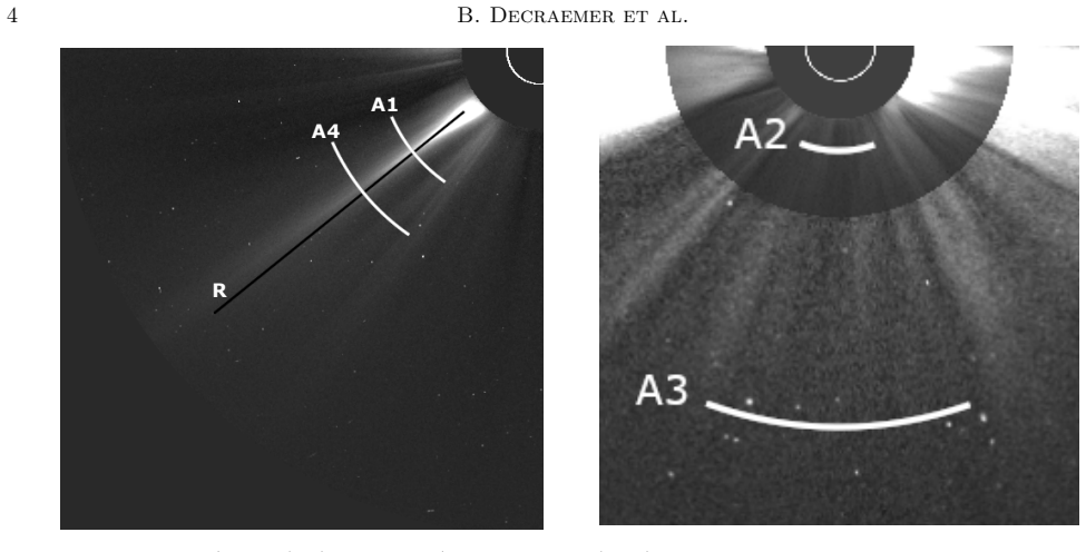
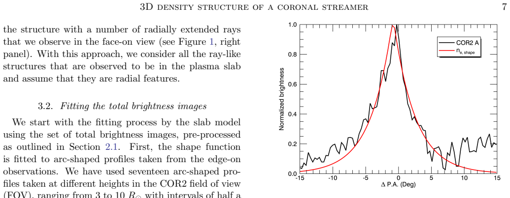
The central device is the separable slab model of the streamer. The electron density is written as the product of three independent functions: a radial profile $n_{e,\mathrm{radial}}(r)$ (a four-term polynomial in $r^{-i}$), a transverse shape function $n_{e,\mathrm{shape}}(r,\theta)$ (a Gaussian-like profile in latitude whose width parameters $\theta_1(r)$ and $\theta_2(r)$ are each polynomials in $r^{-i}$, governing how slab thickness changes with height), and a face-on modulation $n_{e,\mathrm{face}}(\alpha)$ (the normalized brightness profile at 3 $R_\odot$, representing azimuthal density variations along the current sheet). Separability lets each function be fitted to the appropriate brightness profile independently: the shape function to seventeen arc-shaped edge-on profiles, the radial function to one radial brightness profile in the edge-on view, and the face-on function to the azimuthal profile in the face-on view. The fitted density is then integrated along the line of sight with Thomson-scattering forward modeling, so predicted brightness is compared directly with observed brightness in both geometries.
What would settle it
Observe the same streamer from a third vantage point that is not in quadrature with the other two (for instance, from STEREO B on the same date, or from SOHO at a later time if the streamer persists), forward-model the expected brightness using the paper's published density cube, and compare pixel by pixel; if the predicted brightness deviates from the observed image by more than the noise level anywhere outside the fitted slab's symmetry plane, then the slab geometry and the factor-3 ray contrast are falsified as a description of the streamer's true 3D density.
Extended reading notes
Core claim
The discovery is that a helmet streamer's three-dimensional electron density can be represented by a separable slab model, $n_e(r,\alpha,\theta) = n_{e,\mathrm{radial}}(r)\,n_{e,\mathrm{shape}}(r,\theta)\,n_{e,\mathrm{face}}(\alpha)$, with all parameters determined by fitting the model to two quadrature views. The face-on modulation, taken from the brightness profile at 3 $R_\odot$, is essential: it encodes the brighter and darker ray-like streaks that appear in the LASCO face-on view, and without it the model cannot reproduce the observed azimuthal brightness variations. With it, the forward model matches the brightness profiles in both the edge-on COR2 view and the face-on LASCO view, and yields a density cube in which the electron density of bright rays exceeds that of dark lanes by up to about a factor of 3 (or about 1.5 when fitted to polarized brightness data). The two density cubes from total and polarized brightness agree closely, with a correlation coefficient of 0.96, supporting the use of faster-cadence total-brightness images. The authors conclude that the streamer plasma sheet is not a smooth layer but contains ray-like density structure, possibly produced by non-uniform interchange reconnection at the streamer cusp.
Load-bearing premise
The load-bearing premise is that every ray-like brightness variation in the face-on view lies inside a single, flat, radially oriented plasma slab, that the density modulation measured at 3 $R_\odot$ is the same at all heights, and that the slab is symmetric about a fixed radial axis; if any of these fails — for instance if some streaks are polar plumes or structures outside the slab, or if the contrast changes with height — the fitted factor-3 contrast and slab geometry would be artifacts of the assumed geometry rather than properties of the streamer.
Editorial extensions
If this is right
- The published density cube (Tables 1 and 2 parameters) can serve as a ready-made background density model for studying streamer waves, streamer-blowout CMEs, and other transient events in this streamer.
- Because the face-on modulation is the only ingredient that reproduces the ray-like streaks, the fit demonstrates that the streamer's 3D density cannot be radially uniform: the plasma sheet contains density structures aligned with the current sheet.
- The close agreement between total-brightness and polarized-brightness fits (correlation 0.96) indicates that routine, high-cadence total-brightness images can be used for 3D density reconstruction of streamers, at least below about 5 $R_\odot$.
- The model's failure to capture the streamer's slight bend toward the equator shows that non-radial geometries must be included for accurate reconstructions of streamers whose current sheets are not straight.
Reading between the lines
- If the factor-3 ray contrast is typical of streamer plasma sheets, density fluctuations are large enough to affect the local Alfvén speed and the propagation of streamer waves, so wave models assuming a uniform slab may need revision.
- The assumption that the face-on profile at 3 $R_\odot$ holds at every height could be tested by comparing ray contrast in the model against higher-quality observations at other heights; if contrast varies with height, the density cube's extrapolation to 15 $R_\odot$ would need a height-dependent face-on profile.
- The ray-like density pattern could serve as a tracer of reconnection: if non-uniform interchange reconnection fills the plasma sheet, the spacing and contrast of rays in the 3D cube may encode the spatial and temporal history of that reconnection, an idea testable with future high-resolution coronagraphs that cover the gap between EUV imagers and externally occulted coronagraphs.
Signed reviews
Editorial analysis
A structured set of objections, weighed in public.
Referee Report
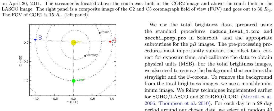
Summary. The manuscript presents a forward model of a helmet streamer observed by SOHO/LASCO and STEREO/COR2 on 2011 April 30 when the two spacecraft were near quadrature. The streamer is modeled as a plasma slab with electron density written as a product of a radial function ne_radial(r), a transverse shape function ne_shape(r,θ), and a face-on modulation ne_face(α). The shape function parameters (b_i, c_i) are fitted to 17 arc-shaped brightness profiles in the edge-on COR2 view; the radial coefficients a_i are fitted to a radial brightness profile in the same view and to an arc profile at 3 R_sun in the face-on LASCO view; ne_face is set equal to the normalized observed azimuthal brightness profile at 3 R_sun. The procedure is repeated for polarized brightness (pB) images. The paper reports density cubes with ray-like structures of contrast up to a factor 3 (total brightness) and about 1.5 (pB), and claims good correspondence with observations.
Significance. The quadrature viewing geometry is a genuinely new observational resource, and the paper is commendable for including forward-modeled views, comparison with previous density models, and an honest discussion of limitations. If the model assumptions were validated, the density cube would be a useful product for studies of streamer waves and slow solar wind. However, the headline result—the factor-3 density contrast—is not an independent outcome of the stereoscopic fit because ne_face is directly taken from the observed face-on profile at 3 R_sun; the 3D extension relies on untested assumptions about radiality and height invariance that the paper itself argues against. These issues must be addressed before the central claim can be accepted.
major comments (4)
- [Section 3.1, Eq. (1)] ne_face is defined as the normalized circular brightness profile at 3 R_sun extracted from the face-on LASCO view, so the forward-modeled face-on profile at 3 R_sun in Fig. 9 reproduces the observation by construction rather than as a test of the model. Consequently, the factor-3 density contrast quoted in the abstract and Section 4.1 is a restatement of the observed brightness modulation at that height, not a quantity constrained by the quadrature fit. The paper should either present ne_face as an input and explicitly discuss the factor-3 value as an observed quantity, or provide an independent validation at other heights (e.g., a quantitative comparison at 11 R_sun, where the paper itself notes mismatches).
- [Section 3.2 and Section 4.2] The 3D density cube and the factor-3 contrast rely on the assumptions that all face-on brightness variations lie inside a single radial slab and that the 3 R_sun profile describes the density modulation at all heights. The manuscript itself provides evidence against both: Section 3.2 states that at 11 R_sun 'not all the variations in the profile correspond to variations that can be seen in the input profile at 3 R_sun' and that 'not all the ray-like structures in the LASCO view are perfectly radial,' and Section 4.2 concedes that some radial features 'may be polar plumes, or the quasi-radial density enhancement ... or other structures in the solar corona' outside the slab. These admissions show that the derived cube is an extrapolation based on premises the paper contradicts; without additional modeling or masking of external features, the factor-3 density contrast cannot be attributed unambiguously to the streamer plasma sheet.
- [Section 3.3, Fig. 12] The pB-derived model does not reproduce the observed LASCO C2 pB azimuthal profile at 3 R_sun; the paper patches this by adding a polar density component from Guhathakurta et al. (1996), but explicitly describes this combined model as 'used here only for illustration' and does not fit it. Therefore the agreement between total and pB density cubes (Fig. 14, correlation 0.96) does not establish that the pB model matches the actual pB observations in the LASCO view, and the abstract's statement that 'densities derived using polarized and unpolarized data are similar' is not fully supported by the presented fits.
- [Tables 1 and 2 and Section 3.2] No uncertainties are reported for the fitted parameters a_i, b_i, c_i, nor are any goodness-of-fit statistics given, so the significance of the factor-3 contrast and of any differences between the total-brightness and pB models cannot be assessed. In addition, the claimed 'simultaneous' multivariate fit is sequential: the shape function is fitted first to the edge-on profiles, and the radial parameters are then fitted with the shape parameters fixed; a genuinely simultaneous fit would account for the covariance between shape and radial parameters and change the error propagation.
minor comments (6)
- [Abstract] 'For the first time, we simultaneously fit the observational data from SOHO and STEREO using a multivariate minimization algorithm' overstates the procedure, which fits the edge-on and face-on data in separate steps rather than in one global minimization; rephrase to avoid implying a single joint fit.
- [Section 2.1] The monthly-minimum background subtraction removes a fraction of the K corona, as acknowledged, but the magnitude of the resulting systematic error on the derived density is not quantified; a simple estimate would help.
- [Section 3.2, Fig. 7] The noted offset of the streamer axis with height is discussed qualitatively, but the paper does not quantify the effect of ignoring this non-radiality on the fitted shape parameters; a bound on the induced error would strengthen the analysis.
- [Section 3.3] The statement that pB data are unsuitable above 5 R_sun due to F-corona polarization is correct, but the paper could state explicitly that the pB density cube is therefore only validated below this height.
- [Tables 1 and 2] The units of the fitted coefficients are not specified; they follow from the polynomial forms in Eqs. (3)–(4), but stating them explicitly would help reproducibility.
- [Section 4.1, Fig. 13] The comparison with Thernisien & Howard (2006) is only against their density range; a brief description of how their model geometry differs from the present slab model would help the reader interpret the comparison.
Circularity Check
The factor-3 ray contrast is the inserted 3 R_sun face-on brightness profile, not an independent stereoscopic prediction.
-
self definitional
[Section 3.1, Eq. (1); Section 4.1, Fig. 13; Section 5 Conclusions]
"Finally, the face-on modulation is expressed by simply inserting the normalized circular profile at 3 R_sun, taken from the face-on brightness along the angular extent of the slab. ... The ne,face function will enhance or reduce the electron density in the plane of the slab (along the current sheet), in order to reproduce the structure with a number of radially extended rays that we observe in the face-on view."
The face-on density modulation ne,face in Eq. (1) is, by the paper's own description, the observed normalized face-on brightness profile at 3 R_sun inserted directly into the density model. Therefore the forward-modeled face-on profile at 3 R_sun in Fig. 9 is not an independent validation: it reproduces the observed azimuthal brightness variations because those variations are the model input. Likewise, the headline result that 'the streamer plasma sheet contains ... ray-like structures with the density contrast up to about a factor 3' is essentially the observed 3 R_sun face-on brightness contrast restated as a density contrast, not a quantity determined by the stereoscopic fit.
full rationale
The derivation is partially circular. The separable slab model ne = ne,radial * ne,shape * ne,face gives genuinely independent content in the edge-on fitting: the radial density falloff and the slab shape are fitted to COR2 data, the total-brightness and pB models are compared, and the 11 R_sun comparison is a real, if imperfect, out-of-sample test. However, the paper's central claim about ray-like structures and their factor-3 density contrast rests on ne,face, which is explicitly the observed normalized face-on brightness profile at 3 R_sun inserted into the model. Reproducing the face-on profile at 3 R_sun is therefore by construction, and the factor-3 ray contrast is a restatement of the input brightness contrast rather than an independent stereoscopic finding. The paper's own caveats that some face-on features may be polar plumes or out-of-slab structures, and that not all rays are radial, further weaken the extrapolation from that inserted profile to the 3D density cube. No load-bearing self-citation chain or imported uniqueness theorem is present; the circularity is localized to the face-on modulation and the resulting ray-contrast claim.
Assumptions & free parameters
free parameters (6)
- Radial density polynomial coefficients a_i =
Total brightness fit: a1=1.736e5, a2=-2.999e4, a3=5.762e6, a4=9.699e7; pB fit in Table 2
- Shape polynomial coefficients b_i for theta1 =
Total brightness fit: -87.79, 1105, -4785, 8035, -4967; pB fit in Table 2
- Shape polynomial coefficients c_i for theta2 =
Total brightness fit: 3.927, -3.623, 136.4, -1064, 2409; pB fit in Table 2
- Face-on modulation profile at 3 R_sun =
Normalized observed azimuthal brightness profile, not tabulated
- Streamer central position angle for the fit =
128.17 degrees
- Slab angular extent in Carrington longitude =
40 degrees
assumptions (5)
- domain assumption White-light coronal brightness is dominated by Thomson scattering and is a line-of-sight integral over electron density.
- ad hoc to paper The streamer is a single plasma slab centered on a current sheet, and all ray-like structures lie inside that slab and are radial.
- ad hoc to paper The streamer slab is oriented orthogonal to the plane of the sky in the COR2 view, so projection effects can be neglected when fitting the shape function.
- ad hoc to paper The face-on profile at 3 R_sun represents the azimuthal density structure at all heights, because the rays are radial.
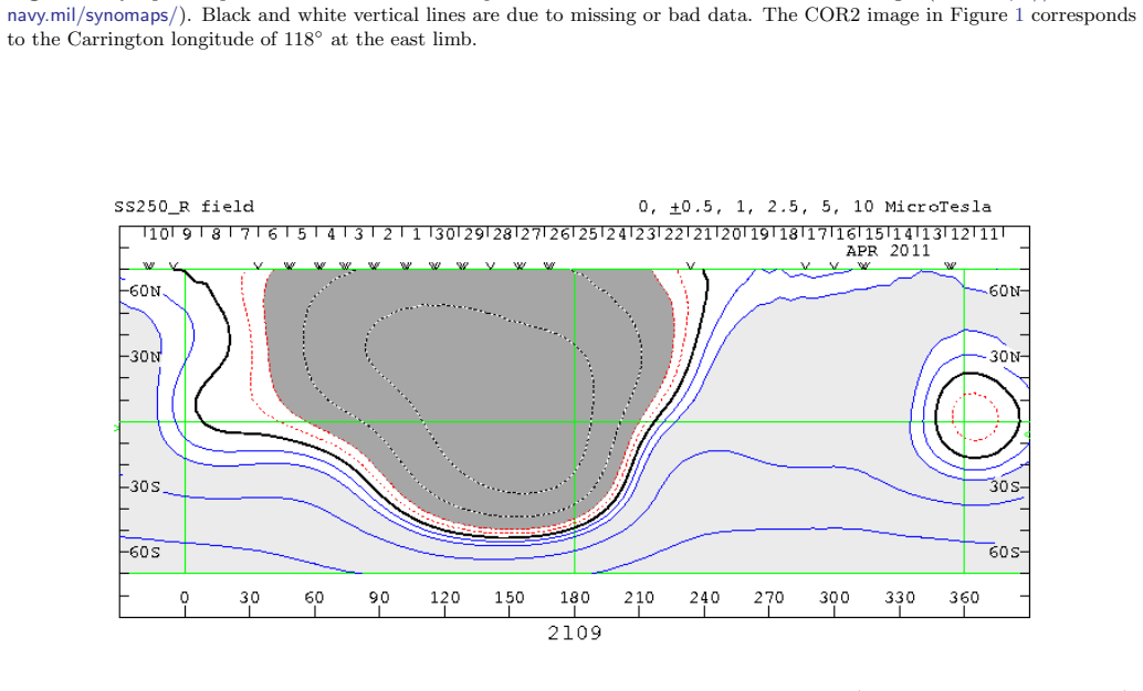
- domain assumption The PFSS extrapolation locates the heliospheric current sheet neutral line accurately enough to place the slab.
Cite this review
Pith. "Pith review of Three-dimensional Density Structure of a Solar Coronal Streamer Observed by SOHO/LASCO and STEREO/COR2 in Quadrature." pith.science (2026). https://pith.science/paper/BDHUHRCH
@misc{pith2026190805034,
  author       = {Pith},
  title        = {Pith review of: Three-dimensional Density Structure of a Solar Coronal Streamer Observed by SOHO/LASCO and STEREO/COR2 in Quadrature},
  year         = {2026},
  howpublished = {\url{https://pith.science/paper/BDHUHRCH}},
  note         = {Machine review of arXiv:1908.05034}
}
read the original abstract
Helmet streamers are a prominent manifestation of magnetic structures with current sheets in the solar corona. These large-scale structures are regions with high plasma density, overlying active regions and filament channels. We investigate the three-dimensional (3D) structure of a coronal streamer, observed simultaneously by white-light coronagraphs from two vantage points near quadrature (SOHO/LASCO and STEREO/COR2). We design a forward model based on plausible assumptions about the 3D streamer structure taken from physical models (a plasma slab centered around a current sheet). The streamer stalk is approximated by a plasma slab, with electron density that is characterized by three separate functions describing the radial, transverse and face-on profiles respectively. For the first time, we simultaneously fit the observational data from SOHO and STEREO using a multivariate minimization algorithm. The streamer plasma sheet contains a number of brighter and darker ray-like structures with the density contrast up to about a factor 3 between them. The densities derived using polarized and unpolarized data are similar. We demonstrate that our model corresponds well to the observations.
Figures

Figures from the paper (12 more)


Reference graph
Works this paper leans on
-
[1]
Aschwanden, M. J. 2011, LRSP, 8, 5, doi: 10.12942/lrsp-2011-5
-
[2]
Aschwanden, M. J., Nitta, N. V., Wuelser, J.-P., & Lemen, J. R. 2008a, ApJ, 680, 1477, doi: 10.1086/588014
-
[3]
Aschwanden, M. J., W¨ ulser, J.-P., Nitta, N. V., & Lemen, J. R. 2008b, ApJ, 679, 827, doi: 10.1086/529542
-
[4]
Brueckner, G. E., Howard, R. A., Koomen, M. J., et al. 1995, SoPh, 162, 357, doi: 10.1007/BF00733434
-
[5]
Chen, Y., Song, H. Q., Li, B., et al. 2010, ApJ, 714, 644, doi: 10.1088/0004-637X/714/1/644
-
[6]
DeForest, C. E., Howard, T. A., & Tappin, S. J. 2013, ApJ, 765, 44, doi: 10.1088/0004-637X/765/1/44
-
[7]
Elmore, D. F., Burkepile, J. T., Darnell, J. A., Lecinski, A. R., & Stanger, A. L. 2003, in Society of Photo-Optical Instrumentation Engineers (SPIE) Conference Series, Vol. 4843, Proc. SPIE, ed. S. Fineschi, 66–75
work page 2003
-
[8]
Eselevich, V. G., & Eselevich, M. V. 1999, SoPh, 188, 299, doi: 10.1023/A:1005150721459
Show all 46 references
-
[9]
W., Chen, Y., Li, B., et al
Feng, S. W., Chen, Y., Li, B., et al. 2011, SoPh, 272, 119, doi: 10.1007/s11207-011-9814-6
2011 doi
-
[10]
A., Lamy, P., Llebaria, A., & V´ asquez, A
Frazin, R. A., Lamy, P., Llebaria, A., & V´ asquez, A. M. 2010, SoPh, 265, 19, doi: 10.1007/s11207-010-9557-9
2010 doi
-
[11]
2018, in Society of Photo-Optical Instrumentation Engineers (SPIE) Conference Series, Vol
Galano, D., Bemporad, A., Buckley, S., et al. 2018, in Society of Photo-Optical Instrumentation Engineers (SPIE) Conference Series, Vol. 10698, Space Telescopes and Instrumentation 2018: Optical, Infrared, and Millimeter Wave, 106982Y
2018
-
[12]
E., Foster, D
Gibson, S. E., Foster, D. J., Guhathakurta, M., Holzer, T., & St. Cyr, O. C. 2003, J. Geophys. Res., 108, 1444, doi: 10.1029/2003JA009994
2003 doi
-
[13]
E., & MacQueen, R
Guhathakurta, M., Holzer, T. E., & MacQueen, R. M. 1996, ApJ, 458, 817, doi: 10.1086/176860
1996 doi
-
[14]
P., Vourlidas, A., & Howard, R
Hayes, A. P., Vourlidas, A., & Howard, R. A. 2001, ApJ, 548, 1081, doi: 10.1086/319029
2001 doi
-
[15]
K., Antiochos, S
Higginson, A. K., Antiochos, S. K., DeVore, C. R., Wyper, P. F., & Zurbuchen, T. H. 2017, ApJ, 837, 113, doi: 10.3847/1538-4357/837/2/113
2017 doi
-
[16]
A., Moses, J
Howard, R. A., Moses, J. D., Vourlidas, A., et al. 2008, SSRv, 136, 67, doi: 10.1007/s11214-008-9341-4
2008 doi
-
[17]
2016, arXiv e-prints, arXiv:1512.00651v2
Inhester, B. 2016, arXiv e-prints, arXiv:1512.00651v2. https://arxiv.org/abs/1512.00651v2
2016 arXiv
-
[18]
L., Kucera, T
Kaiser, M. L., Kucera, T. A., Davila, J. M., et al. 2008, SSRv, 136, 5, doi: 10.1007/s11214-007-9277-0
2008 doi
-
[19]
J., Howard, R
Koomen, M. J., Howard, R. A., & Michels, D. J. 1998, SoPh, 180, 247, doi: 10.1023/A:1005039609265
1998 doi
-
[20]
1971, A&A, 13, 79
Koutchmy, S. 1971, A&A, 13, 79
1971
-
[21]
Koutchmy, S., & Lamy, P. L. 1985, in IAU Colloq. 85: Properties and Interactions of Interplanetary Dust, ed. R. H. Giese & P. Lamy, 63
1985
-
[22]
1992, SSRv, 61, 393, doi: 10.1007/BF00222313
Koutchmy, S., & Livshits, M. 1992, SSRv, 61, 393, doi: 10.1007/BF00222313
1992 doi
-
[23]
2010, in Society of Photo-Optical Instrumentation Engineers (SPIE) Conference Series, Vol
Lamy, P., Dam´ e, L., Viv` es, S., & Zhukov, A. 2010, in Society of Photo-Optical Instrumentation Engineers (SPIE) Conference Series, Vol. 7731, Proc. SPIE, 773118
2010
-
[24]
A., & Bougeret, J.-L
Leblanc, Y., Dulk, G. A., & Bougeret, J.-L. 1998, SoPh, 183, 165, doi: 10.1023/A:1005049730506
1998 doi
-
[25]
L., & Koutchmy, S
Loucif, M. L., & Koutchmy, S. 1989, A&AS, 77, 45
1989
-
[26]
Markwardt, C. B. 2009, in Astronomical Society of the Pacific Conference Series, Vol. 411, Astronomical Data Analysis Software and Systems XVIII, ed. D. A
2009
-
[27]
2009, SoPh, 259, 123, doi: 10.1007/s11207-009-9416-8 16 B
Mierla, M., Inhester, B., Marqu´ e, C., et al. 2009, SoPh, 259, 123, doi: 10.1007/s11207-009-9416-8 16 B. Decraemer et al
2009 doi
-
[28]
2015, ApJS, 219, 23, doi: 10.1088/0067-0049/219/2/23 —
Morgan, H. 2015, ApJS, 219, 23, doi: 10.1088/0067-0049/219/2/23 —. 2019, ApJS, 242, 3, doi: 10.3847/1538-4365/ab125d
2015 doi
-
[29]
Morgan, H., & Habbal, S. R. 2007, A&A, 464, 357, doi: 10.1051/0004-6361:20066482
2007 doi
-
[30]
S., Korendyke, C
Morrill, J. S., Korendyke, C. M., Brueckner, G. E., et al. 2006, SoPh, 233, 331, doi: 10.1007/s11207-006-2058-1
2006 doi
-
[31]
1967, ARA&A, 5, 213, doi: 10.1146/annurev.aa.05.090167.001241 Qu´ emerais, E., & Lamy, P
Newkirk, Gordon, J. 1967, ARA&A, 5, 213, doi: 10.1146/annurev.aa.05.090167.001241 Qu´ emerais, E., & Lamy, P. 2002, A&A, 393, 295, doi: 10.1051/0004-6361:20021019
1967
-
[32]
2015, in Society of Photo-Optical Instrumentation Engineers (SPIE) Conference Series, Vol
Renotte, E., Alia, A., Bemporad, A., et al. 2015, in Society of Photo-Optical Instrumentation Engineers (SPIE) Conference Series, Vol. 9604, Proc. SPIE, 96040A
2015
-
[33]
2007, A&A, 473, 265, doi: 10.1051/0004-6361:20066777
Saez, F., Llebaria, A., Lamy, P., & Vibert, D. 2007, A&A, 473, 265, doi: 10.1051/0004-6361:20066777
2007 doi
-
[34]
N., Lamy, P., & Llebaria, A
Saez, F., Zhukov, A. N., Lamy, P., & Llebaria, A. 2005, A&A, 442, 351, doi: 10.1051/0004-6361:20042016
2005 doi
-
[35]
I., & Munro, R
Saito, K., Poland, A. I., & Munro, R. H. 1977, SoPh, 55, 121, doi: 10.1007/BF00150879
1977 doi
-
[36]
Thernisien, A., Vourlidas, A., & Howard, R. A. 2009, SoPh, 256, 111, doi: 10.1007/s11207-009-9346-5
2009 doi
-
[37]
F., & Howard, R
Thernisien, A. F., & Howard, R. A. 2006, ApJ, 642, 523, doi: 10.1086/500818
2006 doi
-
[38]
F., Patel, N
Thernisien, A. F., Patel, N. S., Howard, R. A., Marqu´ e, C., & Vourlidas, A. 2004, in AGU Fall Meeting Abstracts, Vol. 2004, SH21B–0404
2004
-
[39]
Thernisien, A. F. R., Howard, R. A., & Vourlidas, A. 2006, ApJ, 652, 763, doi: 10.1086/508254
2006 doi
-
[40]
T., Wei, K., Burkepile, J
Thompson, W. T., Wei, K., Burkepile, J. T., Davila, J. M., & St. Cyr, O. C. 2010, SoPh, 262, 213, doi: 10.1007/s11207-010-9513-8 van de Hulst, H. C. 1950, BAN, 11, 135 V´ asquez, A. M., Frazin, R. A., Hayashi, K., et al. 2008, ApJ, 682, 1328, doi: 10.1086/589682 V´ asquez, A. ...
2010 doi
-
[41]
1997, in ESA Special
Vibert, D., Lamy, P., & Liebaria, A. 1997, in ESA Special
1997
-
[42]
Vourlidas, A., & Webb, D. F. 2018, ApJ, 861, 103, doi: 10.3847/1538-4357/aaca3e
2018 doi
-
[43]
Wang, Y. M. 1996, ApJ, 456, L119, doi: 10.1086/309871 —. 2002, AdSpR, 30, 491, doi: 10.1016/S0273-1177(02)00323-X
1996 doi
-
[44]
M., Sheeley, N
Wang, Y. M., Sheeley, N. R., J., & Rich, N. B. 2000a, Geophys. Res. Lett., 27, 149, doi: 10.1029/1999GL010698 —. 2007, ApJ, 658, 1340, doi: 10.1086/511416
2007 doi
-
[45]
M., Sheeley, N
Wang, Y. M., Sheeley, N. R., Socker, D. G., Howard, R. A., & Rich, N. B. 2000b, J. Geophys. Res., 105, 25133, doi: 10.1029/2000JA000149
-
[46]
2008, ApJ, 680, 1532, doi: 10.1086/587924
Stenborg, G. 2008, ApJ, 680, 1532, doi: 10.1086/587924
2008 doi
Reviewed August 14, 2026 · model on record in the stance chip above.
Discussion (0). Continue with ORCID to comment.