REVIEW 2 major objections 6 minor 70 references
Two-fluid simulations of waves in the solar chromosphere II. Propagation and damping of fast magneto-acoustic waves and shocks
T0 review · 2 major / 6 minor · reviewed 2026-08-14 · deepseek-v4-flash
Pith's one-line read The damping of fast magneto-acoustic waves in the solar chromosphere is set by linear ion–neutral decoupling, and shock steepening dramatically amplifies it.
desk verdict A careful two-fluid wave-damping study whose linear part is well supported by a WKB comparison, and whose nonlinear-heating conclusion needs a grid-convergence check before it is fully convincing. read the letter →
The pith
A machine-rendered reading of the paper's core claim, the machinery that carries it, and where it could break.
The reading
What carries the argument
The central object is a two-fluid system for a hydrogen plasma with ionized charges and neutrals coupled by elastic collisions. The momentum exchange is $\mathbf{R}_n = \alpha \rho_n \rho_c(\mathbf{u}_c-\mathbf{u}_n)$ and the energy exchange contains a frictional heating term $\tfrac12\alpha\rho_n\rho_c(\mathbf{u}_c-\mathbf{u}_n)^2$ plus thermal exchange, with the collisional parameter $\alpha$ built from ion-neutral and electron-neutral collision frequencies. The argument is carried by a WKB (slowly varying amplitude) solution of the linearized two-fluid equations, which reduces the problem to a fourth-order dispersion relation in the vertical wavenumber $k$; the imaginary part of $k$ as a function of height gives the damping length. The decisive comparison is between the simulated wave amplitude and this analytic WKB amplitude, which separates linear decoupling effects from nonlinear shock effects.
What would settle it
The paper itself shows that raising the collisional coefficient by a factor of $10^4$ eliminates decoupling; the claim would be falsified if a two-fluid simulation with realistically strong coupling still showed comparable damping, or if the analytic WKB damping failed to track the linear numerical solution in the same stratified hydrogen atmosphere. A concrete test is to measure the height where a 1 s fast wave is damped in the strong-field profile and compare it with the height at which the imaginary part of the WKB wavenumber becomes negative; a mismatch larger than the WKB approximation error would indicate another damping mechanism.
Extended reading notes
Core claim
On the paper's own terms, the central discovery is that the amplitude loss of fast magneto-acoustic waves in a stratified, partially ionized chromosphere is governed by the linear decoupling of the charged and neutral fluids. The evidence is the close match between numerical solutions of the linearized two-fluid equations and an analytic WKB solution of the same system; the WKB solution's imaginary wavenumber gives the damping length. Because this agreement holds before shocks form, the paper attributes the damping to linear effects; in the nonlinear regime, the same collisional term acts on the shortened spatial scales of shock fronts, so shock steepening strongly increases the damping. The decoupling height responds sensitively to wave period, amplitude, and field strength, and the frictional heating term raises the background temperature at a steady rate proportional to the square of the velocity difference.
Load-bearing premise
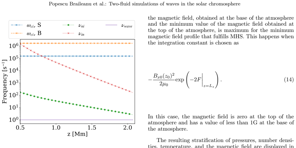
The central conclusions stand on the assumed collisional coupling between charges and neutrals, set by fixed cross sections in a hydrogen-only atmosphere; if the real chromospheric collision frequencies differ, the decoupling heights, damping lengths, and heating rates all move.
Editorial extensions
If this is right
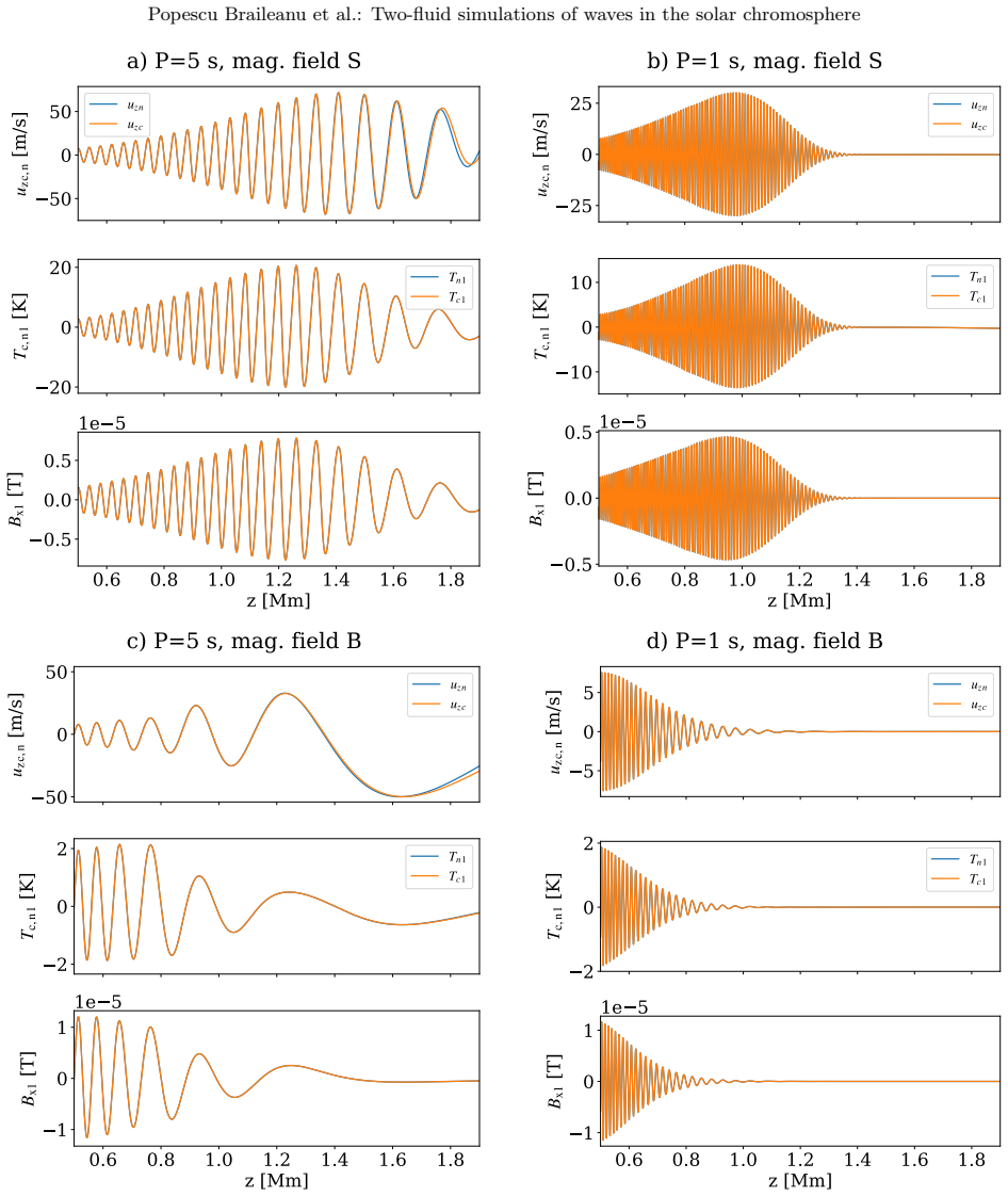
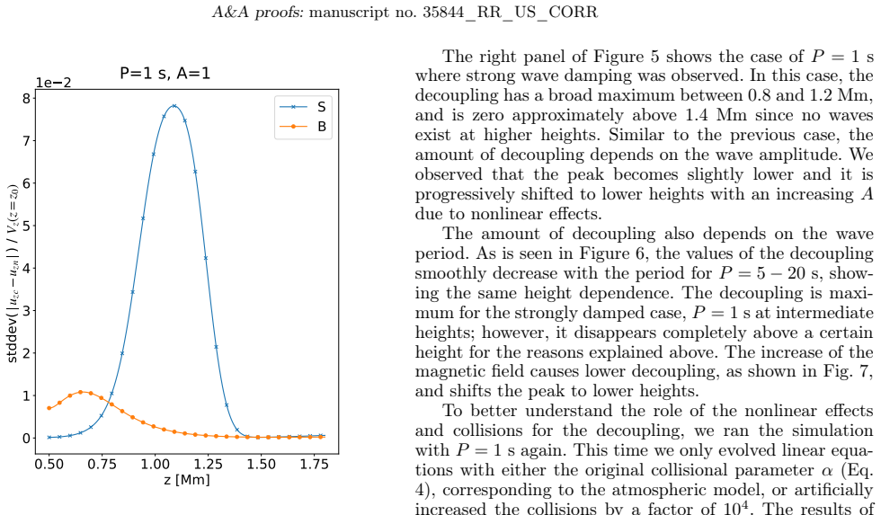
- High-frequency waves (periods 1–5 s) are damped within the modeled chromosphere; in the stronger-field profile a 1 s wave essentially disappears by about 0.8 Mm.
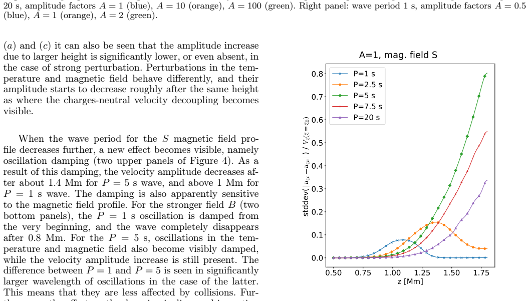
- The height where decoupling begins falls as the wave period decreases and as the magnetic field strengthens, yet the damping length is shorter for the weaker field.
- Frictional heating accumulates linearly in time, raising the temperature of both fluids and reducing the background magnetic field, at a rate proportional to the squared velocity difference.
- In the linear regime the analytic WKB solution matches the simulations closely, indicating that reflection and nonlinearities are not needed to explain the damping.
- Nonlinear shock steepening markedly increases collisional damping, and the effect is stronger for shorter-period waves because their shocks form at lower heights.
Reading between the lines
- If the collision cross sections are revised, the decoupling heights, damping lengths, and heating rates shift systematically; observed damping of high-frequency chromospheric waves could therefore serve as a constraint on the ion-neutral collision frequency.
- Because the control run with artificially increased collisions eliminates decoupling, the same setup offers a clean numerical testbed for any future code that adds ionization, radiation, or conduction: those additions should preserve the linear WKB damping baseline if the present claim is right.
- The 1D horizontal-field geometry likely understates the role of shock-front geometry; in multi-dimensional simulations with inclined fields, the effective front scale varies along the front, which would spread the damping over a range of heights rather than a single sharp layer.
Editorial analysis
A structured set of objections, weighed in public.
Referee Report
Summary. The paper presents two-fluid simulations of fast magneto-acoustic waves in a stratified, purely hydrogen model of the solar chromosphere, using the MANCHA3D code. Waves are driven at the base of the chromosphere for periods 1–20 s and amplitude factors A = 0.5–100, in two horizontal magnetic-field profiles. The authors quantify the height-dependent decoupling between ion and neutral velocities, the associated collisional damping, and frictional heating. They derive a WKB solution of the linearized two-fluid equations and compare it with linear and nonlinear numerical runs. The principal claims are that (i) in the linear regime the damping is well described by the WKB solution and arises from ion-neutral decoupling, and (ii) nonlinear steepening dramatically increases collisional damping. Time-averaged temperature increases are attributed to frictional heating.
Significance. If fully established, the paper would provide a useful quantitative framework for two-fluid damping and heating of chromospheric fast waves, including a WKB tool for estimating linear damping and a separation of linear and nonlinear contributions. The model is transparent, the governing equations are given explicitly, and the linear comparison (Fig. 14) and the α×10^4 control (Fig. 8) are strong internal consistency checks. However, the nonlinear part of the central claim currently rests on runs without shock capturing and without a grid-convergence study, so the enhanced damping in Fig. 16 could be partly numerical. The quantitative outputs also depend on fixed collision cross sections, and no sensitivity study is presented. These issues are addressable with additional numerical experiments.
major comments (2)
- [Section 4.1 (Fig. 16; Fig. 3 caption)] The conclusion that nonlinear steepening "dramatically increases" collisional damping is not yet numerically secured. The nonlinear runs are performed with a second-order scheme that, as the authors explicitly note for the A=100 cases (Fig. 3 caption), produces shock-overshoot artifacts because no shock-capturing algorithm is used. Since the A=10 runs in Fig. 16 also develop saw-tooth wave fronts, they are likely subject to the same numerical deficiency. No grid-convergence study is reported, and the paper does not demonstrate that the numerical dissipation at unresolved shock fronts is small compared with the physical collisional dissipation. The frictional-heating term Q ∝ (u_c−u_n)^2 in Eq. (25) amplifies spurious small-scale velocity differences at under-resolved fronts, so the enhanced amplitude decay in Fig. 16 and the temperature increase in Figs. 9–11 could be contaminated by numerical heating. Please provide a convergence study at two additional grid resolutions for a representative case (e.g., A=10, P=5 s) or a comparison with a shock-capturing/artificial-viscosity variant, and quantify the numerical contribution to the heating budget.
- [Section 2.1 (Eqs. 4–5) and Section 4.1] The quantitative results—decoupling heights, damping lengths, and heating rates—scale directly with the collision frequencies in Eq. (5), which adopt fixed cross sections σ_in = 5×10^−19 m^2 and σ_en = 10^−19 m^2 from Braginskii (1965). The only collisional sensitivity test is the α×10^4 control in Fig. 8, which is an extreme strong-coupling limit rather than a realistic uncertainty range. Because the paper makes specific quantitative statements (e.g., decoupling above 0.7–1 Mm, damping lengths for 1 s and 5 s waves), the authors should test the robustness of these heights and damping lengths to a factor-of-two variation in α (or in the cross sections). Without such a test, it is unclear how much of the quantitative output is an artifact of the assumed momentum-transfer cross sections.
minor comments (6)
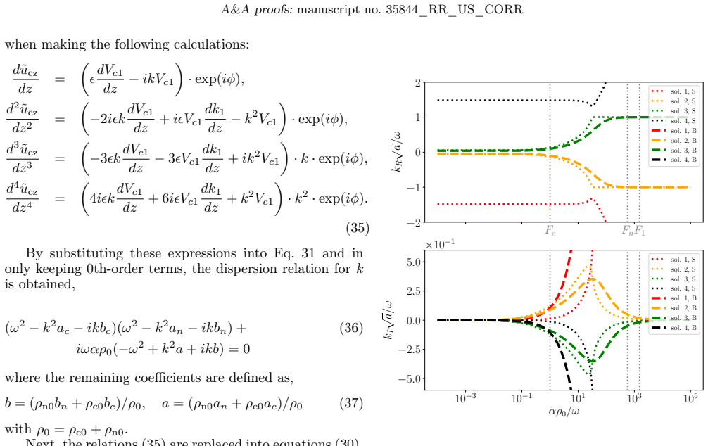
- [Equation (35)] Equation (35) appears to contain a systematic typo: the terms proportional to −ik and −k^2 are written with V_{c1}(z) in place of the full amplitude V_c(z) (or V_{c0} at zeroth order). As printed, the zeroth-order terms would vanish and the dispersion relation (36) would not follow; I assume this is a typesetting error, but it should be corrected to make the derivation traceable.
- [Section 2.1, after Eq. (5)] The sentence "Additionally, both temperatures are assumed to be equal to Tc" is ambiguous: the model has separate T_n and T_c, and Eq. (3) includes a thermal exchange term (T_c−T_n). Presumably the authors mean that the initial equilibrium temperatures of charges and neutrals are equal; please clarify.
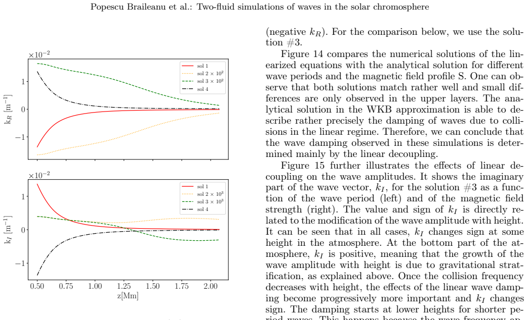
- [Section 4.1, Fig. 14] The WKB analytical solution is derived from the same linearized two-fluid equations and the same background atmosphere as the numerical runs, so the agreement in Fig. 14 is an internal consistency check rather than an independent validation. The paper should state this explicitly, so that readers do not overinterpret the comparison as a benchmark against an external model.
- [Section 2.2, Eq. (13)] The description of the integration constant C and the role of the parameter j (S-profile vs B-profile) is terse; the sentence "The integration constant dominates over the space-varying term" is difficult to follow. Please expand the explanation of how the two magnetic-field profiles are constructed and why the constant term makes the field almost flat.
- [Figure 12] The text refers to modes #1 and #4 as "unphysical" in the strongly coupled limit, but the criterion for this classification is not stated. Please define the criterion (e.g., extremely large k_I/k_R, or negative group velocity) so the reader can interpret the solution branches.
- [Section 3.2, Fig. 9] The statement that a temperature increase of about 0.5 K "is not negligible" relative to the 10 K oscillation amplitude would benefit from a dimensionless measure (e.g., a heating rate per wave period or a fraction of the local temperature), which is available in Fig. 10 and the text.
Circularity Check
No significant circularity; the WKB comparison is an internal consistency check, not a fitted prediction.
full rationale
The paper's central claims are extracted from numerical evolution of the two-fluid equations, and the analytical WKB solution is derived independently from the linearized versions of the same equations and the same background atmosphere. No free parameter is fitted to the simulation output in the comparison shown in Fig. 14: the analytical solution uses the same boundary velocity amplitude, wave frequency, and background collision frequencies as the runs, so it can fail to match the numerical solution in shape, height of damping onset, or damping length. The close agreement therefore tests whether the linear numerical solver implements the same physics as the WKB reduction, which is a legitimate consistency check rather than a circular prediction. The decoupling height and damping onset are emergent quantities; they are not used to define any input parameter. The control run with the collision parameter multiplied by 10^4 (Fig. 8) is a genuine parameter variation and the nonlinear-versus-linear comparison in Fig. 16 separates regimes without renaming fitted data. Self-citations to Popescu Braileanu et al. (2019) and the Braginskii (1965) cross sections support code implementation and physical inputs, respectively, and are not load-bearing for the target conclusion. The acknowledged absence of shock-capturing algorithms for the A=100 cases is a numerical accuracy risk for the nonlinear-damping conclusion, but it is a correctness concern, not circularity.
Assumptions & free parameters
free parameters (4)
- Base magnetic field strength Bx0(z0) =
1e-4 T
- Magnetic field integration constant C =
0.988 Pa (S profile), 120.73 Pa (B profile)
- Wave amplitude factor A =
0.5, 1, 2, 10, 100
- Wave period P =
1, 2.5, 5, 7.5, 20 s
assumptions (4)
- domain assumption The solar plasma can be described as two distinct fluids, charges (ions plus electrons) and neutrals, with only elastic collisional coupling; no ionization/recombination, viscosity, thermal conduction, or radiation are included.
- domain assumption A pure hydrogen plasma is a valid model for the upper photosphere and chromosphere, with metal electrons neglected; the VALC temperature profile is used but densities are recomputed for hydrogen.
- domain assumption The WKB approximation is valid: wavelengths are shorter than the stratification scale and amplitude/wavenumber gradients are small (Eq. 34).
- domain assumption The driver at the lower boundary is accurately represented by the linearized single-fluid solution with ambipolar diffusion neglected at the bottom (Eqs. 17-22).
Cite this review
Pith. "Pith review of Two-fluid simulations of waves in the solar chromosphere II. Propagation and damping of fast magneto-acoustic waves and shocks." pith.science (2026). https://pith.science/paper/EJRBKX4G
@misc{pith2026190805262,
  author       = {Pith},
  title        = {Pith review of: Two-fluid simulations of waves in the solar chromosphere II. Propagation and damping of fast magneto-acoustic waves and shocks},
  year         = {2026},
  howpublished = {\url{https://pith.science/paper/EJRBKX4G}},
  note         = {Machine review of arXiv:1908.05262}
}
read the original abstract
Waves and shocks traveling through the solar chromospheric plasma are influenced by its partial ionization and weak collisional coupling, and may become susceptible to multi-fluid effects, similar to interstellar shock waves. In this study, we consider fast magneto-acoustic shock wave formation and propagation in a stratified medium, that is permeated by a horizontal magnetic field, with properties similar to that of the solar chromosphere. The evolution of plasma and neutrals is modeled using a two-fluid code that evolves a set of coupled equations for two separate fluids. We observed that waves in neutrals and plasma, initially coupled at the upper photosphere, become uncoupled at higher heights in the chromosphere. This decoupling can be a consequence of either the characteristic spatial scale at the shock front, that becomes similar to the collisional scale, or the change in the relation between the wave frequency, ion cyclotron frequency, and the collisional frequency with height. The decoupling height is a sensitive function of the wave frequency, wave amplitude, and the magnetic field strength. We observed that decoupling causes damping of waves and an increase in the background temperature due to the frictional heating. The comparison between analytical and numerical results allows us to separate the role of the nonlinear effects from the linear ones on the decoupling and damping of waves.
Figures


Figures from the paper (12 more)





Reference graph
Works this paper leans on
-
[1]
Anderson , L. S. and Athay , R. G. 1989, , 336, 1089
work page 1989
- [2]
-
[3]
L., Alexeev , I., Collados , M., et al
Ballester , J. L., Alexeev , I., Collados , M., et al. 2018 a , , 214, 58
work page 2018
-
[4]
L., Carbonell , M., Soler , R., and Terradas , J
Ballester , J. L., Carbonell , M., Soler , R., and Terradas , J. 2018 b , , 609, A6
work page 2018
-
[5]
Bello Gonz \'a lez , N., Flores Soriano , M., Kneer , F., and Okunev , O. 2009, , 508, 941
work page 2009
-
[6]
Bello Gonz \'a lez , N., Flores Soriano , M., Kneer , F., Okunev , O., and Shchukina , N. 2010 a , , 522, A31
work page 2010
-
[7]
Bello Gonz \'a lez , N., Franz , M., Mart \' nez Pillet , V., et al. 2010 b , , 723, L134
work page 2010
-
[8]
1994, Journal of Computational Physics, 114, 185
Berenger , J.-P. 1994, Journal of Computational Physics, 114, 185
work page 1994
Show all 70 references
-
[9]
J., Carlsson , M., Hansteen , V
Bogdan , T. J., Carlsson , M., Hansteen , V. H., et al. 2003, , 599, 626
2003
-
[10]
Braginskii , S. I. 1965, Reviews of Plasma Physics, 1, 205
1965
-
[11]
Cally , P. S. 2006, Philosophical Transactions of the Royal Society of London Series A, 364, 333
2006
-
[12]
Cally , P. S. and Goossens , M. 2008, , 251, 251
2008
-
[13]
and Stein , R
Carlsson , M. and Stein , R. F. 2002, in ESA Special Publication, Vol. 505, SOLMAG 2002. Proceedings of the Magnetic Coupling of the Solar Atmosphere Euroconference, ed. H. Sawaya-Lacoste , 293--300
2002
-
[14]
Cheung , M. C. M. and Cameron , R. H. 2012, , 750, 6
2012
-
[15]
Draine , B. T. 1980, , 241, 1021
1980
-
[16]
Draine , B. T. and McKee , C. F. 1993, , 31, 373
1993
-
[17]
T., Roberge , W
Draine , B. T., Roberge , W. G., and Dalgarno , A. 1983, , 264, 485
1983
-
[18]
2010, , 719, 357
Felipe , T., Khomenko , E., and Collados , M. 2010, , 719, 357
2010
-
[19]
and Carlsson , M
Fossum , A. and Carlsson , M. 2006, , 646, 579
2006
-
[20]
Gupta , G. R. 2014, AandA, 568, A96
2014
-
[21]
2016, , 591, A112
Hillier , A., Takasao , S., and Nakamura , N. 2016, , 591, A112
2016
-
[22]
and Tripathi , D
Isobe , H. and Tripathi , D. 2006, AandA, 449, L17
2006
-
[23]
B., Mathioudakis , M., Erd \'e lyi , R., et al
Jess , D. B., Mathioudakis , M., Erd \'e lyi , R., et al. 2008, , 680, 1523
2008
-
[24]
B., Morton , R
Jess , D. B., Morton , R. J., Verth , G., et al. 2015, , 190, 103
2015
-
[25]
2017, Plasma Physics and Controlled Fusion, 59, 014038
Khomenko , E. 2017, Plasma Physics and Controlled Fusion, 59, 014038
2017
-
[26]
and Calvo Santamaria , I
Khomenko , E. and Calvo Santamaria , I. 2013, in Journal of Physics Conference Series, Vol. 440, Journal of Physics Conference Series, 012048
2013
-
[27]
and Collados , M
Khomenko , E. and Collados , M. 2006, , 653, 739
2006
-
[28]
and Collados , M
Khomenko , E. and Collados , M. 2009, , 506, L5
2009
-
[29]
and Collados , M
Khomenko , E. and Collados , M. 2012, , 747, 87
2012
-
[30]
and Collados , M
Khomenko , E. and Collados , M. 2015, Living Reviews in Solar Physics, 12, 6
2015
-
[31]
2014 a , Physics of Plasmas, 21, 092901
Khomenko , E., Collados , M., D \' az , A., and Vitas , N. 2014 a , Physics of Plasmas, 21, 092901
2014
-
[32]
2014 b , , 565, A45
Khomenko , E., D \' az , A., de Vicente , A., Collados , M., and Luna , M. 2014 b , , 565, A45
2014
-
[33]
2017, , 604, A66
Khomenko , E., Vitas , N., Collados , M., and de Vicente , A. 2017, , 604, A66
2017
-
[34]
2018, ArXiv e-prints
Khomenko , E., Vitas , N., Collados , M., and de Vicente , A. 2018, ArXiv e-prints
2018
-
[35]
A., Tanner , S
Klimchuk , J. A., Tanner , S. E. M., and De Moortel , I. 2004, , 616, 1232
2004
-
[36]
E., DeVore , C
Leake , J. E., DeVore , C. R., Thayer , J. P., et al. 2014, , 184, 107
2014
-
[37]
S., and Linton , M
Lee , E., Lukin , V. S., and Linton , M. G. 2014, AandA, 569, A94
2014
-
[38]
and Zhang , J
Li , T. and Zhang , J. 2012, , 760, L10
2012
-
[39]
Luna , M., Terradas , J., Oliver , R., and Ballester , J. L. 2008, , 676, 717
2008
-
[40]
G., Alvarez Laguna , A., Lani , A., and Poedts , S
Maneva , Y. G., Alvarez Laguna , A., Lani , A., and Poedts , S. 2017, , 836, 197
2017
-
[41]
2016, , 832, 101
Mart \' nez-G \'o mez , D., Soler , R., and Terradas , J. 2016, , 832, 101
2016
-
[42]
2017, , 837, 80
Mart \' nez-G \'o mez , D., Soler , R., and Terradas , J. 2017, , 837, 80
2017
-
[43]
2016, , 831, L1
Mart \' nez-Sykora, J., De Pontieu, B., Carlsson, M., and Hansteen, V. 2016, , 831, L1
2016
-
[44]
2012, , 753, 161
Mart \' nez-Sykora , J., De Pontieu , B., and Hansteen , V. 2012, , 753, 161
2012
-
[45]
A., De Moortel , I., Hood , A
McLaughlin , J. A., De Moortel , I., Hood , A. W., and Brady, C. S. 2009, AandA, 493, 227
2009
-
[46]
Mullan , D. J. 1971, , 153, 145
1971
-
[47]
E., Rosner , R., Stein , R
Musielak , Z. E., Rosner , R., Stein , R. F., and Ulmschneider , P. 1994, , 423, 474
1994
-
[48]
Nye , A. H. and Thomas , J. H. 1976, , 204, 573
1976
-
[49]
Sehgal, a
Ofman, L., Nakariakov, V., and N. Sehgal, a. 2008, , 533, 1071
2008
-
[50]
S., Khomenko , E., and de Vicente , \'A
Popescu Braileanu , B., Lukin , V. S., Khomenko , E., and de Vicente , \'A . 2019, , 627, A25
2019
-
[51]
M., and Lukin , V
Provornikova , E., Laming , J. M., and Lukin , V. S. 2018, ArXiv e-prints
2018
-
[52]
P., Przybylski , D., et al
Rijs , C., Rajaguru , S. P., Przybylski , D., et al. 2016, , 817, 45
2016
-
[53]
C., Khomenko , E., Collados , M., and de Vicente , A
Santamaria , I. C., Khomenko , E., Collados , M., and de Vicente , A. 2017, , 602, A43
2017
-
[54]
2016, , 819, L11
Shelyag , S., Khomenko , E., de Vicente , A., and Przybylski , D. 2016, , 819, L11
2016
- [55]
-
[56]
L., and Terradas , J
Soler , R., Carbonell , M., Ballester , J. L., and Terradas , J. 2013 a , , 767, 171
2013
-
[57]
J., Ballester , J
Soler , R., Díaz , A. J., Ballester , J. L., and Goossens , M. 2013 b , AandA, 551, A86
2013
-
[58]
and Terradas , J
Soler , R. and Terradas , J. 2015, , 803, 43
2015
-
[59]
Soler , R., Terradas , J., Oliver , R., and Ballester , J. L. 2017, , 840, 20
2017
-
[60]
and Vasyli \= u nas , V
Song , P. and Vasyli \= u nas , V. M. 2011, Journal of Geophysical Research (Space Physics), 116, A09104
2011
-
[61]
V., et al
Tóth, G., van der Holst, B., Sokolov, I. V., et al. 2012, Journal of Computational Physics, 231, 870 , special Issue: Computational Plasma PhysicsSpecial Issue: Computational Plasma Physics
2012
-
[62]
Vasquez , B. J. 2005, Journal of Geophysical Research (Space Physics), 110, A10S02
2005
-
[63]
E., Avrett , E
Vernazza , J. E., Avrett , E. H., and Loeser , R. 1981, , 45, 635
1981
-
[64]
M., Ofman , L., and Deluca , E
Verwichte , E., Nakariakov , V. M., Ofman , L., and Deluca , E. E. 2004, , 223, 77
2004
-
[65]
Withbroe , G. L. and Noyes , R. W. 1977, Annual Review of Astronomy and Astrophysics, 15, 363
1977
-
[66]
V., Khodachenko , M
Zaqarashvili , T. V., Khodachenko , M. L., and Rucker, H. O. 2011, AandA, 529, A82
2011
-
[67]
V., Khodachenko , M
Zaqarashvili , T. V., Khodachenko , M. L., and Soler , R. 2013 a , , 549, A113
2013
-
[68]
V., Khodachenko , M
Zaqarashvili , T. V., Khodachenko , M. L., and Soler , R. 2013 b , , 549, A113
2013
-
[69]
, " * write output.state after.block = add.period write newline
ENTRY address author booktitle chapter edition editor howpublished institution journal key month note number organization pages publisher school series title type volume year label extra.label sort.label short.list INTEGERS output.state before.all mid.sentence after.sentence a...
-
[70]
write newline
" write newline "" before.all 'output.state := FUNCTION n.dashify 't := "" t empty not t #1 #1 substring "-" = t #1 #2 substring "--" = not "--" * t #2 global.max substring 't := t #1 #1 substring "-" = "-" * t #2 global.max substring 't := while if t #1 #1 substring * t #2 gl...
Reviewed August 14, 2026 · model on record in the stance chip above.
Discussion (0). Continue with ORCID to comment.