REVIEW 4 major objections 5 minor 20 references
A hierarchical model for estimating exposure-response curves from multiple studies
T0 review · 4 major / 5 minor · reviewed 2026-08-14 · deepseek-v4-flash
Pith's one-line read Pooling three cookstove studies through a hierarchical Bayesian model yields a common exposure-response curve that rises between 50 and 200 µg/m³ of PM2.5 and flattens above that.
desk verdict A careful, genuinely useful methods paper for pooling exposure-response data, but the headline empirical finding is not as solid as the abstract implies because the common-curve assumption is doing a lot of work. read the letter →
The pith
A machine-rendered reading of the paper's core claim, the machinery that carries it, and where it could break.
The reading
What carries the argument
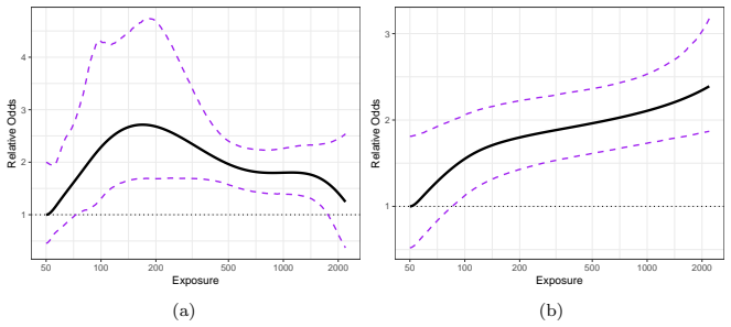
The load-bearing machinery is the two-level hierarchical model itself. The exposure level models each log-transformed PM measurement as a normal draw around a household mean built from stove-group, cluster, and household random effects with a B-spline time trend, which is what lets sparse longitudinal measurements borrow strength across households and clusters. The outcome level models ALRI counts as binomial with a logit link, using I-splines—a monotone spline basis whose non-negative coefficients force a non-decreasing exposure-response curve—to map assigned long-term exposure to disease odds; a shared coefficient vector across studies implements the common-curve assumption, and an LKJ prior (a single-hyperparameter prior on correlation matrices) allows study-specific curves as a sensitivity analysis. At the center of the linkage is the assigned exposure $x_{it}$, computed as a 28-day average of the posterior mean household concentration excluding the time trend, which converts the exposure model's output into a usable regressor while intentionally trading classical error for Berkson error.
What would settle it
Re-fit the combined analysis with the exposure-response coefficients free to vary by study and compare the posterior distributions of the three curves: if the study-specific curves diverge beyond the shrinkage allowed by the LKJ prior, the common-curve assumption behind the primary result fails. A complementary test would randomize households to interventions that move measured PM2.5 within the 50–200 $\mu$g/m$^3$ range and record ALRI incidence; the pooled curve predicts a detectable increase in odds across that interval, whereas a flat curve would refute it.
Extended reading notes
Core claim
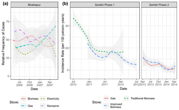
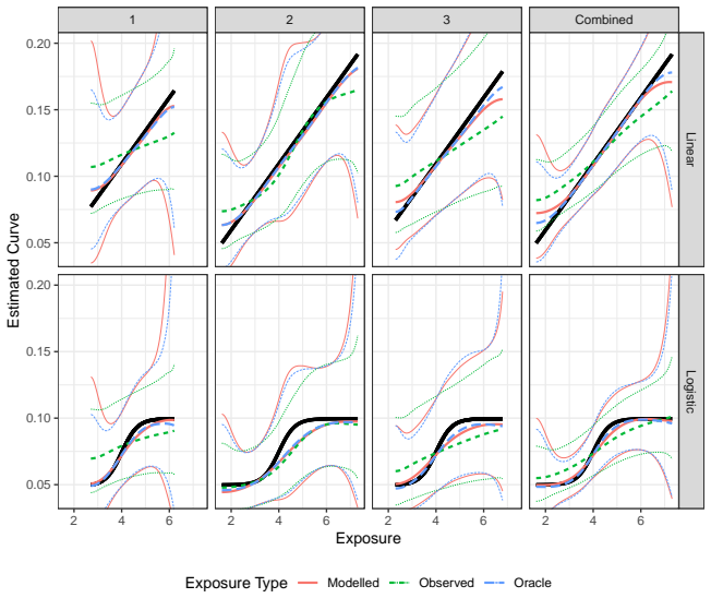
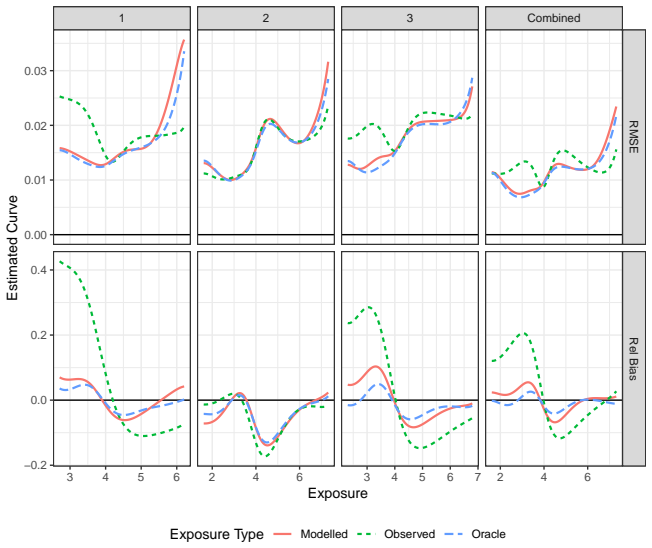
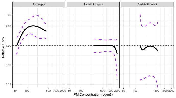
The paper's central claim is that a two-stage hierarchical model can recover a common exposure-response curve from heterogeneous studies. In the first stage, log PM2.5 measurements are modeled separately within each study using stove-group, cluster, and household random effects plus a smooth time trend, so households with one or two observations are shrunk toward group means. In the second stage, each child's assigned long-term exposure—the 28-day average of the posterior mean household concentration, excluding the time trend—enters a logistic outcome model whose exposure term is an I-spline basis with coefficients shared across studies, allowing only study-level intercepts to differ. The fitted joint curve shows the odds of ALRI increasing over the 50 to 200 $\mu$g/m$^3$ range and flattening above it; the monotone-restricted version continues to rise slightly at high concentrations, while the unrestricted version declines where data are sparse. Simulations support the design choice by showing that the shrinkage-based exposure estimates reduce error in household long-term averages and that pooling studies narrows uncertainty in the pooled curve.
Load-bearing premise
The pooled curve assumes the same underlying exposure-response relationship holds in all three studies once study-specific baseline illness rates are allowed, even though the studies differ in design, population, susceptibility, outcome ascertainment, and exposure measurement; if that exchangeability fails, the pooled curve is a weighted average that may represent no single study.
Editorial extensions
If this is right
- If the common curve is correct, cookstove interventions that lower PM2.5 from very high levels to around 200 $\mu$g/m$^3$ should produce little detectable reduction in childhood ALRI, while reductions from 200 toward 50 $\mu$g/m$^3$ should produce the largest benefit.
- Burden-of-disease calculations can replace a parametric curve fit to a single household-air-pollution study with a semi-parametric curve estimated jointly from case-control, step-wedge, and parallel-trial data.
- The framework is designed to absorb additional cookstove studies as they appear: each study's exposure model is fit separately to avoid instrument and measurement differences, while the outcome stage pools information across studies.
- Because exposure contrasts largely shrink to stove-group means, pooling studies that cover different concentration ranges is what makes the full curve identifiable; no single study in this application spans enough of the range to estimate it alone.
Reading between the lines
- The authors leave implicit that the flattening, if causal, makes the distribution of achieved concentrations—not just the average reduction—the key design target for cookstove programs, since health gains would concentrate almost entirely below about 200 $\mu$g/m$^3$.
- The curve is estimated from three Nepal populations; pooling studies from other regions with different co-pollutant mixes or disease epidemiology could reveal whether the plateau is a general property of PM2.5 toxicity or a feature of this setting.
- Using the posterior mean of exposure rather than the full posterior is an approximation; a fully joint Bayesian fit might sharpen or widen the low-exposure slope depending on how much exposure-model uncertainty is currently ignored.
- A testable extension would be to run the same machinery on kitchen concentrations of other pollutants (for example carbon monoxide) from the same studies to see whether the 50–200 $\mu$g/m$^3$ signal is specific to PM2.5 or reflects a broader kitchen-air effect.
Signed reviews
Editorial analysis
A structured set of objections, weighed in public.
Referee Report
Summary. This paper proposes a hierarchical Bayesian two-stage approach for estimating an exposure-response curve by pooling data from multiple cookstove studies. The exposure component models sparse, clustered, longitudinal PM2.5 measurements with household and cluster random effects and temporal splines, fitted separately for each study; the outcome component uses a binomial/logistic model with I-spline exposure-response terms, study intercepts, time splines, and subject random effects. The primary pooled analysis assumes a single exposure-response coefficient vector across studies, with a sensitivity analysis allowing study-specific coefficients. The method is applied to three Nepali studies (Bhaktapur case-control, Sarlahi Phase 1 step-wedge, Sarlahi Phase 2 parallel trial). Simulations show that shrinkage improves estimates of household long-term exposure and that modeled exposures yield better curve estimates than raw observed exposures. The headline applied finding is evidence of increased ALRI odds between roughly 50 and 200 ug/m3 with flattening at higher concentrations.
Significance. If the central claims held, the paper would make a useful methodological contribution: it offers a principled way to combine heterogeneous studies with measurement error, a semi-parametric monotone exposure-response curve, and reproducible software (the bercs R package). The simulation studies provide concrete evidence that shrinkage can improve long-term exposure estimates and that pooling reduces curve uncertainty. However, the applied conclusion is currently under-supported because it rests on an exchangeability assumption that is not validated, and because key sensitivity analyses are too weak to adjudicate between-study heterogeneity. The manuscript is therefore valuable as a modeling framework but needs stronger evidence or a more cautious framing before the headline finding can be accepted.
major comments (4)
- [Section 4.2 and Section 6.3] The primary pooled analysis assumes a single exposure-response coefficient vector beta across all studies. This assumption is load-bearing for the headline claim. The Bhaktapur study shows a steep increase in odds in the 50-200 ug/m3 range, while Sarlahi Phase 2, which covers the overlapping range of roughly 186-395 ug/m3, shows no dose-response relationship. The pooled curve is therefore a weighted average of discordant study-specific curves, and the manuscript itself notes large pointwise uncertainty between 100 and 300 ug/m3 due to contrasting evidence. The sensitivity analysis allowing study-specific beta produces very wide credible intervals because each study spans only a narrow portion of the shared spline basis, so it cannot establish that a common curve is appropriate. Please provide a formal assessment of heterogeneity (for example, comparison of study-specific curves in the overlapping exposure range, a heterogeneity statistic, or an interaction test) and either temper the conclusion or justify the exchangeability assumption more convincingly.
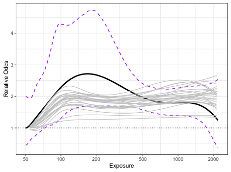
- [Section 4.4 and Section 6.4] The two-stage approach replaces the exposure variable with the posterior mean E[eta_gki | w] and does not propagate the full exposure-model uncertainty into the outcome model. The sensitivity analysis in Section 6.4 is informal: it examines only 25 posterior draws and reports that curves are 'slightly attenuated' without providing a quantitative measure of attenuation or changes in interval coverage. Because the central applied claim concerns a specific exposure range, the uncertainty statements in Figure 7 should be backed by a more principled propagation of exposure uncertainty, such as multiple imputation across posterior draws with Rubin's rules or a comparison of interval widths under the posterior-mean approximation versus full propagation.
- [Section 6.2 and Discussion] The Sarlahi Phase 1 step-wedge study is acknowledged to be confounded: large temporal trends mean that only cross-sectional contrasts identify the exposure-response relationship, and the difference in exposure between stove types is confounded with temporal trends in exposure values. This study provides most of the information at concentrations above roughly 500 ug/m3, so the claim of flattening or a decline at higher exposures rests heavily on a design with limited internal validity. A sensitivity analysis that excludes Phase 1, or otherwise demonstrates that the high-exposure portion of the curve is not driven by the confounded study, is needed before the flattening claim can be considered robust.
- [Section 5] The simulation validation is generated from the same model family that is fitted to the data, so it does not test robustness to model misspecification or to the key exchangeability assumption. In particular, no simulation examines a setting in which the true exposure-response curve differs by study, even though this is the main threat to the primary pooled analysis. Adding such a misspecification scenario, or a simulation with a different true curve shape, would strengthen the claim that the framework is flexible and robust.
minor comments (5)
- [Abstract and Section 6.3] The abstract states 'We find evidence of increased odds of disease for particulate matter concentrations between 50 and 200 ug/m3' without noting that this result depends on the common-curve assumption. The conclusion should be explicitly qualified in the abstract and in Section 6.3.
- [Section 6.2] The sentence 'Because of the step-wedge design, this limits the information available for estimating the exposure-response effect to the period in which only part of the cohort had received the improved stoves' is phrased awkwardly; it would be clearer to say that the information is limited to cross-sectional contrasts during the step-wedge transition period.
- [Table 3 caption] The caption says 'posterior means ... and estimated pooling factors are each level of the exposure model'; 'are' should be 'at'.
- [References] The Carroll et al. reference contains a typo ('2nd editio edition'), and the Supplemental Material statement 'available on request' should be updated to include the repository or URL.
- [Figure 4 caption] The caption refers to 'lightweight lines' for credible intervals; 'light' or 'thin' would be clearer.
Circularity Check
No circularity: the exposure-response curve is estimated from data via a hierarchical two-stage model, and no input is defined in terms of the claimed output.
full rationale
The paper's central claim is an empirical estimate, not a derivation from first principles. The exposure model is fit to measured PM2.5 concentrations separately for each study, and the outcome model regresses ALRI outcomes on posterior-mean exposure summaries. The estimated exposure-response curve is the fitted surface of the outcome model; no equation defines a target quantity in terms of another target quantity, and no fitted parameter is renamed as an independent prediction. The two-stage use of posterior means is explicitly acknowledged as an approximation in Section 4.4 and explored by sensitivity analysis in Section 6.4, which does not create circularity. The self-citations (Bates et al. 2013/2018, Tielsch et al. 2014) are data sources rather than load-bearing methodological support; the statement that the Bhaktapur curve is consistent with Bates et al. (2018) is a corroborating observation, not an input to the model. Simulations are generated from the same model family, so they demonstrate internal consistency rather than external validity, but that is a validation limitation, not circularity. The exchangeability assumption of a single coefficient vector across studies is a modeling assumption, not a circular step. No load-bearing step reduces to its own inputs.
Assumptions & free parameters
free parameters (5)
- I-spline boundary and interior knots =
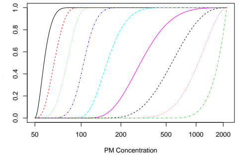
Boundary: 50, 2200; interior: 60, 85, 100, 125, 200, 500 µg/m3
- Exposure averaging window (T-tilde) =
28 days
- Time spline degrees of freedom in outcome model =
8
- Prior hyperparameters for variance components =
Half-normal with m_j, v_j; N+(0,1) for some σ
- Exposure model spline degrees of freedom =
Not explicitly specified in main text
assumptions (5)
- domain assumption The log-transformed PM2.5 measurements follow a normal distribution with household and cluster random effects.
- ad hoc to paper A single exposure-response curve (up to study-specific intercepts) applies across the three studies.
- domain assumption The posterior mean of the exposure model is an adequate substitute for the full posterior distribution of long-term exposure in the outcome model.
- domain assumption Temporal trends in disease risk and exposure are adequately captured by the spline bases used.
- domain assumption The exposure-response function is monotone non-decreasing in the constrained model.
Cite this review
Pith. "Pith review of A hierarchical model for estimating exposure-response curves from multiple studies." pith.science (2026). https://pith.science/paper/E4D6TQOH
@misc{pith2026190805340,
  author       = {Pith},
  title        = {Pith review of: A hierarchical model for estimating exposure-response curves from multiple studies},
  year         = {2026},
  howpublished = {\url{https://pith.science/paper/E4D6TQOH}},
  note         = {Machine review of arXiv:1908.05340}
}
abstract
Cookstove replacement trials have found mixed results on their impact on respiratory health. The limited range of concentrations and small sample sizes of individual studies are important factors that may be limiting their statistical power. We present a hierarchical approach to modeling exposure concentrations and pooling data from multiple studies in order to estimate a common exposure-response curve. The exposure concentration model accommodates temporally sparse, clustered longitudinal observations. The exposure-response curve model provides a flexible, semi-parametric estimate of the exposure-response relationship while accommodating heterogeneous clustered data. We apply this model to data from three studies of cookstoves and respiratory infections in children in Nepal, which represent three study types: crossover trial, parallel trial, and case-control study. We find evidence of increased odds of disease for particulate matter concentrations between 50 and 200 $\mu$g/m$^3$ and a flattening of the exposure-response curve for higher exposure concentrations. The model we present can incorporate additional studies and be applied to other settings.
Figures

Figures from the paper (5 more)
Reference graph
Works this paper leans on
-
[1]
Bates, M. N., Chandyo, R. K., Valentiner-Branth, P., Pokhrel, A. K., Mathisen, M., Basnet, S., Shrestha, P. S., Strand, T. A., and Smith, K. R. (2013). Acute lower respiratory infection in childhood and household fuel use in Bhaktapur, Nepal. Environmental Health Perspectives, 121(5):637–642
work page 2013
-
[2]
Bates, M. N., Pokhrel, A. K., Chandyo, R. K., Valentiner-Branth, P., Mathisen, M., Basnet, S., Strand, T. A., Burnett, R. T., and Smith, K. R. (2018). Kitchen PM2.5concentrations and child acute lower respiratory infection in
work page 2018
-
[3]
Environmental Research, 161(March 2017):546–553
Bhaktapur, Nepal: The importance of fuel type. Environmental Research, 161(March 2017):546–553
work page 2017
-
[4]
Turner, M. C., Gapstur, S. M., Diver, W. R., and Cohen, A. (2014). An inte- grated risk function for estimating the global burden of disease attributable to ambient fine particulate matter exposure. Environmental Health Perspectives, 122(4):397–403
work page 2014
-
[5]
Carroll, R. J., Ruppert, D., Stefanski, L. A., and Crainiceanu, C. M. (2006). Measurement Error in Nonlinear Models . Chapman & Hall/CRC, Boca Ra- ton, 2nd editio edition
work page 2006
-
[6]
Naeher, L. P., Rodes, C. E., Vette, A. F., and Balbus, J. M. (2013). Health and Household Air Pollution from Solid Fuel Use: The Need for Improved Exposure Assessment. Environmental health perspectives, 121(10):1120–1128
work page 2013
-
[7]
Gelman, A. and Pardoe, I. (2006). Bayesian Measures of Explained Variance and Pooling in Multilevel (Hierarchical) Models. Technometrics, 48(2):241–251
work page 2006
-
[8]
Jack, D., Jindal, S., Kan, H., Mehta, S., Moschovis, P., Naeher, L., Patel, A., Perez-Padilla, R., Pope, D., Rylance, J., Semple, S., and Martin, W. J. 20 (2014). Respiratory risks from household air pollution in low and middle income countries. The Lancet Respiratory Medicine , 2(10):823–860
work page 2014
Show all 20 references
-
[9]
P., Marshall, J
Grieshop, A. P., Marshall, J. D., and Kandlikar, M. (2011). Health and climate benefits of cookstove replacement options. Energy Policy, 39(12):7530–7542
2011
-
[10]
Lewandowski, D., Kurowicka, D., and Joe, H. (2009). Generating random cor- relation matrices based on vines and extended onion method. Journal of Multivariate Analysis , 100(9):1989–2001
2009
-
[11]
Martin, W. J. (2012). Household air pollution is a major avoidable risk factor for cardiorespiratory disease. Chest, 142(5):1308–1315
2012
-
[12]
Crampin, A., Grigg, J., Balmes, J., and Gordon, S. B. (2017). A cleaner burning biomass-fuelled cookstove intervention to prevent pneumonia in chil- dren under 5 years old in rural Malawi (the Cooking and Pneumonia Study): a cluster randomised controlled trial. The Lancet, 389...
2017
-
[13]
K., Bates, M
Pokhrel, A. K., Bates, M. N., Acharya, J., Valentiner-Branth, P., Chandyo, R. K., Shrestha, P. S., Raut, A. K., and Smith, K. R. (2015). PM<inf>2.5</inf> in household kitchens of Bhaktapur, Nepal, using four different cooking fuels. Atmospheric Environment, 113:159–168
2015
-
[14]
Powell, H., Lee, D., and Bowman, A. (2012). Estimating constrained concentration-response functions between air pollution and health. Environ- metrics, 23(3):228–237
2012
-
[15]
Ramsay, J. O. (1988). Monotone Regression Splines in Action. Statistical Sci- ence, 3(4):425–461
1988
-
[16]
Rosenthal, J. (2015). The Real Challenge for Cookstoves and Health: More Evidence. EcoHealth, 12(1):8–11
2015
-
[17]
and Masera, O
Ruiz-Mercado, I. and Masera, O. (2015). Patterns of Stove Use in the Context of FuelDevice Stacking: Rationale and Implications. EcoHealth, 12(1):42–56
2015
-
[18]
R., McCracken, J
Smith, K. R., McCracken, J. P., Weber, M. W., Hubbard, A., Jenny, A., Thomp- son, L. M., Balmes, J., Diaz, A., Arana, B., and Bruce, N. (2011). Effect of reduction in household air pollution on childhood pneumonia in Guatemala (RESPIRE): A randomised controlled trial.The Lancet...
2011
-
[19]
H., and Clasen, T
Chang, H. H., and Clasen, T. (2018). Modeling the potential health bene- fits of lower household air pollution after a hypothetical liquified petroleum 21 gas (LPG) cookstove intervention. Environment International, 111(November 2017):71–79
2018
-
[20]
C., and LeClerq, S
Checkley, W., Mullany, L. C., and LeClerq, S. C. (2014). Designs of two ran- domized, community-based trials to assess the impact of alternative cookstove installation on respiratory illness among young children and reproductive out- comes in rural Nepal. BMC Public Health , 1...
2014
Reviewed August 14, 2026 · model on record in the stance chip above.
Discussion (0). Continue with ORCID to comment.