Gordian complexes of knots and virtual knots given by region crossing changes and arc shift moves

Amrendra Gill; Andrei Vesnin; Madeti Prabhakar

REVIEW 3 major objections 4 minor 16 references

Gordian complexes of knots and virtual knots given by region crossing changes and arc shift moves

T0 review · 3 major / 4 minor · reviewed 2026-08-14 · deepseek-v4-flash

Challenge this review Re-run · record.json Download PDF Read on arXiv ↗ Review JSON

Pith's one-line read The paper builds infinite families of knots, and of virtual knots, whose members are pairwise one local move apart, producing n-simplices for every n in both Gordian complexes.

desk verdict Useful explicit constructions for two Gordian complexes, but the virtual generalization to arbitrary vertices rests on an unjustified connected sum. read the letter →

arxiv 1908.05382 v1 pith:UEGRNC7R submitted 2019-08-15 math.GT

Amrendra Gill , Madeti Prabhakar , Andrei Vesnin This is my paper · ORCID

classification math.GT MSC 57M2557M27

keywords Gordiancomplexregioncrossingchangearcshiftmovevirtualknotssimplicialunknottingoperationf-polynomialaffineindexpolynomial

verification ladder T0 review T1 audit T2 compute T3 formal

The pith

A machine-rendered reading of the paper's core claim, the machinery that carries it, and where it could break.

The reading

The paper builds, for each base knot, an infinite family of knots in which every two members are changed into one another by a single region crossing change; and for each base virtual knot, an infinite family of virtual knots in which every two members are changed into one another by a single arc shift. Because every pair is distance one, each family spans an $n$-simplex in the corresponding Gordian complex for arbitrarily large $n$. The paper proves this directly for every classical knot, and asserts the same for every virtual knot via connected sums with the constructed family. Distinctness is certified by polynomial invariants: the $c_0$ coefficient polynomial for the classical knots and the maximum degree of the $f$-polynomial for the virtual knots. All constructed virtual knots share the same affine index polynomial, so that invariant cannot separate them.

What carries the argument

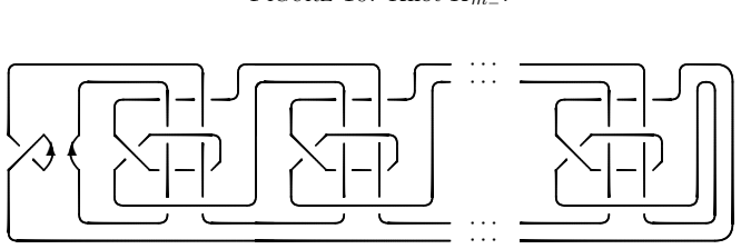
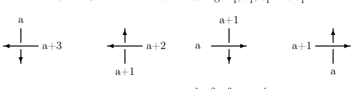
The load-bearing object is the block diagram family together with the invariants that certify distinctness. In the classical case $K_m$ has $m$ copies of one block; region crossing change at the $i$-th region deletes blocks, giving $K_{i-1}$. In the virtual case $VK_n$ has blocks $c_0,\dots,c_n$ made of alternating classical and virtual crossings on a two-strand braid; an arc shift in block $c_j$ frees that braid and cancels all crossings to the right, giving $VK_{j-1}$. Distinctness of $K_m$ is shown through the $c_0$ coefficient polynomial of the skein polynomial, whose degree increases with $m$. Distinctness of $VK_n$ is shown through the bracket polynomial and the normalized $f$-polynomial: a $3\times 3$ transfer matrix tracks the $D$-, $N$-, and $X$-closures of the repeated block, and induction gives maximum $f$-degree $4n$. The paper also labels arcs in $VK_n$ to compute the affine index polynomial, obtaining the common value $2 - t^2 - t^{-2}$ for every $n$.

What would settle it

Take a nontrivial virtual knot $L$ and form $L\sharp VK_1$ using two different choices of connected-sum diagrams or summation arcs; if the two results are inequivalent virtual knots, then the asserted general-vertex statement does not follow from the given construction.

Watch

Extended reading notes

Core claim

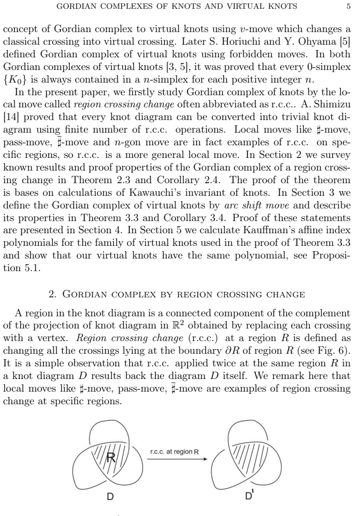
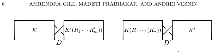
The central discovery is a 'one block per move' diagram family. The knot $K_m$ is built from $m$ identical blocks, and applying a region crossing change at the $i$-th region of $K_m$ returns $K_{i-1}$; hence $K_i$ and $K_j$ are at region-crossing-change distance one for every pair. The virtual knot $VK_n$ is built from $n+1$ blocks, and one arc shift applied to a two-strand braid in block $c_j$ collapses all crossings to its right under the standard diagram moves, returning $VK_{j-1}$; hence all $VK_n$ sit at arc-shift distance one from each other. To know these really are distinct vertices, the paper computes the $c_0$ polynomial for $K_m$, whose maximum degree grows with $m$, and the $f$-polynomial for $VK_n$, whose maximum degree is $4n$. The argument then extends from the unknot to arbitrary knots and virtual knots by connected sum, so every $0$-simplex is contained in an $n$-simplex for every positive $n$.

Load-bearing premise

The argument that the arbitrary-simplex statement passes from the unknot to any virtual knot $L$ assumes that the connected sum $L\sharp VK_i$ is a well-defined virtual knot, independent of chosen diagrams and summation arcs; virtual connected sum is not generally well-defined, and the paper supplies no justification for this step.

Editorial extensions

If this is right

For every classical knot $K_0$, the region-crossing-change Gordian complex contains an $n$-simplex with vertex $K_0$ for every positive integer $n$.
For every virtual knot $L$, the arc-shift Gordian complex is asserted to contain an $n$-simplex with vertex $L$ for every positive integer $n$.
The constructed families form infinite cliques in the distance-one graph of each move: infinitely many pairwise distinct knots that are all one move apart.
Because the region-crossing-change distance between any two classical knots is at most two, the arbitrarily high-dimensional simplices live inside a Gordian complex of diameter at most two.
The common affine index polynomial $2 - t^2 - t^{-2}$ means the arc-shift construction is invisible to that invariant, so it cannot be used to separate members of the family.

Reading between the lines

Editorial extensions of the paper, not claims the author makes directly.

If the virtual connected-sum step can be made well-defined, for instance by using long virtual knots, the arc-shift result would hold for every virtual knot; without such a repair the general-vertex statement is not established by the paper's proof.
The same block-collapse recipe may transfer to other unknotting operations that act locally and kill an entire block, yielding arbitrary-dimensional simplices in their Gordian complexes.
Because all $VK_n$ share one affine index polynomial, it would be informative to test stronger invariants, such as the odd writhe or two-variable $F$-polynomials beyond the range $n \le 10$ checked here.
The paper's boundedness observation for region crossing change suggests that, unlike crossing-change Gordian complexes, high-dimensional simplices here do not imply long geodesic paths; the geometry is concentrated in a two-tier structure.

Share X Bluesky LinkedIn Reddit HN

Signed reviews

No signed human review yet.

Editorial analysis

A structured set of objections, weighed in public.

Desk editor's note, referee report, and a circularity audit.

Desk Editor's Note

read the letter

Read it so you know the construction, but don't trust the corollary.

The paper does something concrete: for the region crossing change on classical knots, it builds explicit knots K_m that are pairwise one r.c.c. apart, and proves they are distinct via Kawauchi's c_0 polynomial. That part is solid. The same template is adapted to virtual knots with the arc shift move, giving VK_n pairwise one arc shift apart, distinguished by the maximum degree of Kauffman's f-polynomial via a tangle-matrix recurrence. That is also plausible; the recurrence is explicit, though there are typos in the printed B matrix and a garbled sign sentence in the affine index section.

The soft spot is Corollary 3.4. The proof is one sentence: connect-sum L with each VK_i. But connected sum of virtual knots is not well-defined on equivalence classes, and the paper neither fixes long or based representatives nor shows the resulting L#VK_i are pairwise distinct. The f-polynomial degree calculation does not transfer, because the f-polynomial of a virtual connected sum is not a simple product when the summand is not classical. Since the abstract advertises arbitrarily high-dimensional simplexes containing any given virtual knot, this gap has to be fixed before publication. It is fixable, but it is not a presentation issue.

Minor quibbles: the max-degree induction for the tangle matrix assumes the degree of a sum of rational functions is the max of the degrees, which can fail by cancellation; the authors should check that the explicit entries do not cancel. The classical connected-sum step in Theorem 2.3 is harmless because classical connected sum is well-defined.

Bottom line: worth a serious referee, but the verdict should be 'revise.' If the authors replace Corollary 3.4 with a statement about long virtual knots, or construct a family directly around L, the paper would be a useful addition to the compendium of Gordian complexes.

Referee Report

3 major / 4 minor

Summary. The manuscript studies two Gordian complexes: the complex of classical knots under region crossing change (r.c.c.) and the complex of virtual knots under arc shift moves. It constructs, for each n, an n-simplex in the r.c.c. Gordian complex containing a prescribed classical knot (Theorem 2.3), and an infinite family of virtual knots that are pairwise at arc-shift distance one (Theorem 3.3). It then claims, in Corollary 3.4, that any virtual knot L is a vertex of an arbitrarily high-dimensional simplex by taking connected sums with the constructed family. Distinctness of the classical family is argued via Kawauchi's coefficient polynomials, and distinctness of the virtual family via maximal degrees of the Kauffman f-polynomial; the paper also computes the affine index polynomial of the virtual knots in Proposition 5.1.

Significance. The constructive approach is concrete and potentially useful, giving explicit infinite cliques in two Gordian complexes. If the virtual-knot extension were proved, the result would nicely parallel known results for the v-move and forbidden-move Gordian complexes. The invariant computations are a genuine strength: Kawauchi's c0 polynomial and the f-polynomial degree method are applied to explicit families rather than asserted abstractly. However, the advertised generalization to an arbitrary virtual knot is not established, because it depends on connected sums of virtual knots without addressing well-definedness or distinctness. The arithmetic error in the degree computation and the unproved cancellation assumption in the max-degree induction are further load-bearing gaps. The unknot-based results are plausible and likely repairable; the arbitrary-virtual-knot claim requires a substantially different argument.

major comments (3)

[Section 4, proof of Corollary 3.4] The proof of Corollary 3.4 is a single sentence asserting that the family {L♯VK_0, ..., L♯VK_n} is the desired simplex. This is not justified. Connected sum of virtual knots is not a well-defined operation on virtual knot isotopy classes: the result generally depends on the chosen diagrams and on the arcs at which the summands are joined. The paper neither fixes representatives nor cites a reference making the operation well-defined in a restricted setting (e.g., long or based virtual knots). Moreover, the proof never shows that the vertices L♯VK_i are pairwise distinct; the f-polynomial degree computation in the proof of Theorem 3.3 applies only to the unsunned VK_n and does not automatically transfer to connected sums with an arbitrary L. Since the abstract explicitly promises an arbitrarily high-dimensional simplex containing any given virtual knot, this gap directly affects the paper's central virtual claim.
[Section 4, Eq. (10) and Proposition 4.2] The computation of the maximum degree of the bracket polynomial of VK_n contains a concrete arithmetic error. Equation (10) states that the max-degree row vector (4,−2,0) times (10n+2, 6n, 10n) gives max degree 10n+6, but the left-hand side evaluates to 4(10n+2) − 2(6n) = 28n+8. This invalidates the stated conclusion that the highest power of the f-polynomial is 4n. Additionally, the 'max' notation used in Proposition 4.2 treats the degree of a sum of products as the maximum of the degrees of the summands; this is an upper bound and can fail by cancellation of leading terms. The proof supplies no check that the relevant leading coefficients do not cancel. The distinctness of the VK_n may be salvageable by a corrected degree computation, but as written the proof is not sound.
[Section 2, proof of Theorem 2.3] The reduction from an arbitrary knot K0 to the unknot is stated in one sentence: 'The general statement will follow by taking connected sums.' For classical knots this can be justified, but the manuscript should spell out the two needed facts: (i) if K_i and K_j differ by one r.c.c. in a region, then K0♯K_i and K0♯K_j differ by one r.c.c. in the corresponding region away from the connected-sum tube, and (ii) the knots K0♯K_i are distinct, which follows from the uniqueness of prime decomposition for classical knots. Without these details, the proof of the advertised 'any knot K0' statement is incomplete, even though the gaps are standard.

minor comments (4)

[Throughout] The manuscript contains many typos and grammatical slips, including 'the exists' in Theorem 2.3, 'bases' in the introduction, 'skien triple' in Section 2, 'Kauffman' for 'Kauffman' in several places, and 'chamge' near the end of Section 2. A careful proofreading pass is needed.
[Section 5, Table 1] The F-polynomial computations are presented only for n = 1,...,10, and the statement that the polynomials are 'the same as for the case n = 3' for n = 4,...,10 is empirical, not a proof for all n. If this discussion is retained, it should be labeled as a finite computation or supplemented with a general argument.
[Section 4, proof of Theorem 3.3] The claim that applying one arc shift move in block c_j of VK_n yields the diagram VK_{j-1} is asserted by inspection of Figures 20 and 21. A more explicit description of the simplification sequence would help the reader verify this key geometric step.
[Section 2, definition of d_R] The definition of the r.c.c. distance is worded confusingly: 'Minimum no. of r.c.c. required to convert all such diagrams D into D'' suggests a minimum over a collection of diagrams without a fully formal quantifier over diagrams of K and K'. A precise definition would improve readability.

Circularity Check

0 steps flagged · score 0.0 of 10

No circularity found: the main simplex constructions are verified by explicit local moves and external invariants, and the connected-sum gap in Corollary 3.4 is a proof omission, not a circular reduction.

full rationale

The paper's central claims are not circular. In Theorem 2.3, the family K_m is shown to have r.c.c. distance one by inspecting the diagram, and distinctness is proved using Kawauchi's c0 polynomial, which is an external skein invariant computed by the stated recurrence rules from [7]; it is not defined in terms of d_R, and no parameter is fitted. In Theorem 3.3, the virtual family VK_n is shown to be pairwise arc-shift distance one by a single arc-shift per block; distinctness is proved by computing the maximum degree of Kauffman's f-polynomial via tangle closures, using Lemma 4.1 from [3] and an explicit B-matrix. The f-polynomial is diagrammatically computed and is not defined in terms of d_A or of the target simplex relation. Section 5's affine index polynomial computation is independent and, as the paper states, does not distinguish the VK_n; the F-polynomial table is exploratory. The self-citations [2] and [11] provide background facts about arc shift moves and polynomial invariants, but the load-bearing construction and invariant computations do not reduce to them, and no uniqueness theorem is imported from the authors' prior work. The only serious weakness is in the one-sentence proof of Corollary 3.4, which passes to L#VK_i without addressing the non-well-definedness of virtual connected sum or proving that the connected sums remain pairwise distinct; this is a correctness or completeness gap concerning virtual knot connected sums, not a circularity by construction. Accordingly, the circularity score is 0.

Assumptions & free parameters 0 free parameters · 6 assumptions · 0 invented entities

The central claims rest on standard invariants and on two external unknotting-operation theorems. The only nonstandard assumption is the well-definedness of virtual connected sum, which is used in Corollary 3.4 and is not established. There are no fitted numerical parameters.

assumptions (6)

domain assumption r.c.c. is an unknotting operation for classical knots
Invoked to define d_R and to assert any two knots can be connected by r.c.c.; from Shimizu [14], cited but not proved in the paper.
domain assumption arc shift move is an unknotting operation for virtual knots
Invoked to define d_A; from the authors' earlier paper [2], cited but not proved.
ad hoc to paper Connected sum of virtual knots is well-defined on isotopy classes
Used in the proof of Corollary 3.4 without justification; virtual knot connected sum is not generally well-defined, so this is an unsupported assumption.
standard math Kawauchi coefficient polynomials c_n satisfy the stated skein rules and c_0(L;1)=1 for knots
Used to distinguish K_m; from Kawauchi [7], standard invariant.
standard math Kauffman f-polynomial is an invariant of virtual knots
Used to distinguish VK_n; from Kauffman [9], standard invariant.
standard math Unique prime decomposition of classical knots
Used implicitly to extend distinctness from K_m to K0#K_m in Theorem 2.3.

how reviews work

0 comments

Cite this review

Pith. "Pith review of Gordian complexes of knots and virtual knots given by region crossing changes and arc shift moves." pith.science (2026). https://pith.science/paper/UEGRNC7R

@misc{pith2026190805382,
  author       = {Pith},
  title        = {Pith review of: Gordian complexes of knots and virtual knots given by region crossing changes and arc shift moves},
  year         = {2026},
  howpublished = {\url{https://pith.science/paper/UEGRNC7R}},
  note         = {Machine review of arXiv:1908.05382}
}

abstract

Gordian complex of knots was defined by Hirasawa and Uchida as the simplicial complex whose vertices are knot isotopy classes in $\mathbb{S}^3$. Later Horiuchi and Ohyama defined Gordian complex of virtual knots using $v$-move and forbidden moves. In this paper we discuss Gordian complex of knots by region crossing change and Gordian complex of virtual knots by arc shift move. Arc shift move is a local move in the virtual knot diagram which results in reversing orientation locally between two consecutive crossings. We show the existence of an arbitrarily high dimensional simplex in both the Gordian complexes, i.e., by region crossing change and by the arc shift move. For any given knot (respectively, virtual knot) diagram we construct an infinite family of knots (respectively, virtual knots) such that any two distinct members of the family have distance one by region crossing change (respectively, arc shift move). We show that that the constructed virtual knots have the same affine index polynomial.

Figures

Figures reproduced from arXiv: 1908.05382 by the authors.

**Figure 1.** H(n)-move. K. Zhang, Z. Yang and F. Lei [16] defined Gordian complex GH(n) of knots by H(n)-move in a similar way by taking all knot isotopy classes as vertex [PITH_FULL_IMAGE:figures/full_fig_p002_1.png] view at source ↗

**Figure 2.** Pass-moves ❄ ✻✲ ✲ ↔ ❄ ✻✲ ✲ ✻ ❄ ✲ ✲ ↔ ✻ ❄ ✲ ✲ [PITH_FULL_IMAGE:figures/full_fig_p003_2.png] view at source ↗

**Figure 3.** #-Moves set and defining a set of n + 1 knots {K0, K1, . . . , Kn} as an n-simplex if dH(n) (Ki , Kj ) = 1 for distinct i and j. It follows that any simplex in GH(n) also forms a simplex in GH(n+1) as a H(n)-move can be realized using one H(n + 1)-move. Further, following results were proved for GH(n) . Theorem 1.4. [16] For any 0-simplex p of the H(n)-Gordian complex, there exists an arbitrarily high dimensional si… view at source ↗

Figures from the paper (31 more)

**Figure 4.** Figure 4: Ck-Move. The [PITH_FULL_IMAGE:figures/full_fig_p004_4.png]

**Figure 5.** Figure 5: #-Move [PITH_FULL_IMAGE:figures/full_fig_p004_5.png]

**Figure 6.** Figure 6: D0 obtained from D by r.c.c. at region R. A. Shimizu [14, Theorem 1.1] proved that a crossing change at any crossing c in a knot diagram D can be realized by applying r.c.c. at finite number of regions in D. Therefore, r.c.c. is an unknotting operation for knots. From …

**Figure 7.** Figure 7: Equivalent diagrams of D and D0 . exist a diagram D such that one r.c.c. in D results in the trivial knot. However, such a diagram D may not always be a minimal diagram of K. Therefore, it may not be always possible to find two minimal diagrams D, D0 of the knots K, K0…

**Figure 8.** Figure 8: Knot Km. dR(Ki , Km) ≤ 1 for i = 0, 1, . . . , m − 1, now varying m from 1 to n we get dR(Ki , Kj ) ≤ 1 for i 6= j ∈ {0, 1, . . . , n}. To show that σn is an n-simplex in GR, it is enough to prove that {Km} n m=0 are distinct knots. In [7] A. Kawauchi introduced the se…

**Figure 9.** Figure 9: Skein triple. Now we consider Km as an oriented knot with the orientation given by vectors presented in [PITH_FULL_IMAGE:figures/full_fig_p007_9.png]

**Figure 10.** Figure 10: Knot Km− . ✻✻ · · · · · · · · · · · · [PITH_FULL_IMAGE:figures/full_fig_p008_10.png]

**Figure 11.** Figure 11: Knot Km0 . ❘✠ · · · · · · · · · · · · [PITH_FULL_IMAGE:figures/full_fig_p008_11.png]

**Figure 12.** Figure 12: Knot Lm. ❄ ❄ ❄ · · · · · · · · · · · · [PITH_FULL_IMAGE:figures/full_fig_p008_12.png]

**Figure 13.** Figure 13: Link Lm0 . Now consider Lm as a knot in a skein triple in respect to the crossing indicated by two vectors in [PITH_FULL_IMAGE:figures/full_fig_p008_13.png]

**Figure 14.** Figure 14: Knot L 0 m. ✛ ✻ · · · · · · · · · · · · [PITH_FULL_IMAGE:figures/full_fig_p009_14.png]

**Figure 15.** Figure 15: Link L 0 m0 . Since linking number of Lm0 is −1 and one of its component is trivial, we have c0(Lm0 ) = x(x − 1) · c0(L 0 m) where by L 0 m we denoted the non-trivial component of Lm0 . This component diagram is presented in [PITH_FULL_IMAGE:figures/full_fig_p009_15.png]

**Figure 16.** Figure 16: Classical and virtual crossings. A virtual crossing is depicted by placing a small circle at the vertex. Two virtual knot diagrams correspond to same virtual knot if one can be obtained from the other via a sequence of generalized Reidemeister moves shown in [PITH_FU…

**Figure 18.** Figure 18: Arc shift on arc (a,b). Arc shift move together with generalized Reidemeister moves is an unknotting operation for virtual knots [2] and hence, any virtual knot K can [PITH_FULL_IMAGE:figures/full_fig_p011_18.png]

**Figure 19.** Figure 19: 2-simplex in GA. In further exploring the simplexes in GA we prove following results which gives us enough examples of simplexes in GA. Theorem 3.3. There exists an infinite family of virtual knots {V Kn}n≥1 such that dA(V Kt , V Ks) = 1 for distinct t, s ≥ 1. As a co…

**Figure 20.** Figure 20: Virtual knot V Kn. 1-simplex in G. Horiuchi et. al. [3] modified this family by changing some of the classical crossings into virtual crossings to show the existence of an n-simplex for each n ∈ N in the Gordian complex of virtual knots by v-move. We add some extra cl…

**Figure 21.** Figure 21: Turning 2-strand braid free of crossings. It is easy to observe from the diagram of V Kn(see [PITH_FULL_IMAGE:figures/full_fig_p013_21.png]

**Figure 22.** Figure 22: A- and B-splits. Loops in a state might have intersections in virtual crossings. L. Kauffman [9] defined bracket polynomial hDi for a diagram D of virtual knot K as follows: hDi = X S A a(S)−b(S) [PITH_FULL_IMAGE:figures/full_fig_p014_22.png]

**Figure 23.** Figure 23: Closures of tangle T [PITH_FULL_IMAGE:figures/full_fig_p014_23.png]

**Figure 24.** Figure 24: Sum T + S of tangles T and S. hDi, where D can be written as D = N(T + S) for some tangles T and S. Lemma 4.1. [3] The following relation holds: hN(T + S)i = (hD(T)i,hN(T)i,hX(T)i) · A · (hD(S)i,hN(S)i,hX(S)i) T , where T denotes the transpose of vector and A is 3 × 3…

**Figure 25.** Figure 25: Tangle T. ❝ ❝ ❝ ❝ ❝ ❝ ❝ ❝ ❝ ❝ ❝ ❝ · · · · · · · · · · · · ❝ ❝ ❝ ❝ ❝ ❝ [PITH_FULL_IMAGE:figures/full_fig_p015_25.png]

**Figure 26.** Figure 26: respectively. From Lemma 4.1, we have hV Kni = hN(T + Sn)i = (hD(T)i,hN(T)i,hX(T)i) · A · (hD(Sn)i,hN(Sn)i,hX(Sn)i) T (2) , ❝ ❝ [PITH_FULL_IMAGE:figures/full_fig_p015_26.png]

**Figure 27.** Figure 27: Virtual links D1, D2 and D3. D4 ❝ ❝ ❝ ❝ ❝ ❝ D5 ❝ ❝ ❝ ❝ ❝ ❝ D6 ❝ ❝ ❝ ❝ ❝ ❝ ❝ [PITH_FULL_IMAGE:figures/full_fig_p016_27.png]

**Figure 28.** Figure 28: Virtual links D4, D5 and D6. D7 ❝ ❝ ❝ ❝ ❝ ❝ ❝ D8 ❝ ❝ ❝ ❝ ❝ ❝ ❝ D9 ❝ ❝ ❝ ❝ ❝ ❝ ❝ ❝ [PITH_FULL_IMAGE:figures/full_fig_p016_28.png]

**Figure 29.** Figure 29: Virtual links D7, D8 and D9. where A is the matrix given in Lemma 4.1. Further, D(Sn) can be seen as N-closure of sum of two tangles by breaking Sn at the dashed line shown in the diagram ( [PITH_FULL_IMAGE:figures/full_fig_p016_29.png]

**Figure 30.** Figure 30: Sign of crossings. ■ ✒ b + 1 a b a − 1 ■ ✒ b + 1 a b a − 1 ■ ✒ ❢ b a b a [PITH_FULL_IMAGE:figures/full_fig_p020_30.png]

**Figure 31.** Figure 31: Labeling of arcs. After labeling assign a weight WD(c) to each classical crossing c defined in [10] as WD(c) = sgn(c)(a − b − 1). Then the Kauffman’s affine index polynomial [10] of virtual knot diagram D is defined as (11) PD(t) = X c∈C(D) sgn(c)(t WD(c) − 1) where t…

**Figure 32.** Figure 32: Labelling in blocks c0 and c1. a a a a ✛ ✲ ✛ ✲ a + 2 a + 1 a + 1 a a + 2 a + 2 a + 2 a + 1 a + 1 a a a a a a a ■ ✒ ■ ✒ ✛ ✲ ✛ ✲ ✛ ✲ c 5 2 c 6 2 c 1 2 c 2 2 c 3 2 c 4 2 ❢ ❢ ❢ ❢ ❢ ❢ · · · · · · · · · · · · a a a a ✛ ✲ ✛ ✲ a + 2 a + 1 a + 1 a a + 2 a + 2 a + 2 a + 1 a + 1…

**Figure 33.** Figure 33: Labelling in blocks c2, . . . , cn. ✛ ❄ a+2 a+3 ✛ ✻ a+1 a+2 ✲ ❄ a+3 a ✲ ✻ a a+1 [PITH_FULL_IMAGE:figures/full_fig_p021_33.png]

**Figure 34.** Figure 34: Labels around crossings c 1 1 , c 2 1 , c 3 1 and c 4 1 . ✛ ❄ a a+3 ✛ ✻ a+1 a+2 ✲ ❄ a+1 a ✲ ✻ a a+1 [PITH_FULL_IMAGE:figures/full_fig_p021_34.png]

**Figure 35.** Figure 35: Labels around crossings c 1 i , c 2 i , c 3 i and c 4 i for i = 2, . . . , n. Summarizing, from all index values computed for classical crossings of V Kn we obtain the affine index polynomial PV Kn (t): (12) PV Kn (t) = sgn(c 1 0 )(t 0 −1)+ sgn(c 2 0 )(t 0 −1)+ X 1≤i≤…

Discussion (0). Continue with ORCID to comment.

Reference graph

Works this paper leans on

16 extracted references · 16 canonical work pages

[1]

Math., 15(1992), 111–121

H.Aida, Unknottingoperationsofpolygonaltype, Tokyo J. Math., 15(1992), 111–121

work page 1992
[2]

A. Gill, K. Kaur and M. Prabhakar, Arc shift number and region arc shift number for virtual knots,J. Korean Math. Soc.56(4) (2019) pp. 1063–1081

work page 2019
[3]

Horiuchi, K

S. Horiuchi, K. Komura, Y. Ohyama and M. Shimozawa, The Gordian complex of virtual knots,Journal of Knot Theory and Its Ramiﬁcations21(14) (2012) 11pp

work page 2012
[4]

Hoste, Y

J. Hoste, Y. Nakanishi and K. Taniyama, Unknotting operations involving trivial tan- gles, Osaka J. Math.27(3) (1990) 555–566

work page 1990
[5]

Horiuchi, Y

S. Horiuchi, Y. Ohyama, The Gordian complex of virtual knots by forbidden moves, Journal of Knot Theory and Its Ramiﬁcations22(9) (2013) 11pp

work page 2013
[6]

Hirasawa, Y

M. Hirasawa, Y. Uchida, The Gordian complex of knots,Journal of Knot Theory and Its Ramiﬁcations11(3) (2002) 363–368

work page 2002
[7]

Kawauchi, On coeﬃcient polynomials of the skein polynomial of an oriented link, Kobe J

A. Kawauchi, On coeﬃcient polynomials of the skein polynomial of an oriented link, Kobe J. Math.11(1) (1994) 49–68

work page 1994
[8]

L. H. Kauﬀman, On Knots,Annals of Mathematics Studies, Vol. 115 (Princeton Uni- veristy Press, Princeton, 1987)

work page 1987

Show all 16 references

[9]

L. H. Kauﬀman, Virtual knot theory,European J. Combin., 20(7) (1999) 663–690

1999
[10]

L. H. Kauﬀman, An aﬃne index polynomial invariant of virtual knots,Journal of Knot Theory and its Ramiﬁcations22(4) (2013) 30 pp. 1340007

2013
[11]

K. Kaur, M. Prabhakar and A. Vesnin, Two-variable polynomial invariants of vir- tual knots arising from ﬂat virtual knot invariants,Journal of Knot Theory and its Ramiﬁcations27(13) (2018) 22 pp. 1842015

2018
[12]

Murakami, Some metrics on classical knots,Math

H. Murakami, Some metrics on classical knots,Math. Ann.270 (1985) 35–45

1985
[13]

Ohyama, The Ck-Gordian complex of knots, Journal of Knot Theory and Its Ramiﬁcations15(1) (2006) 73–80

Y. Ohyama, The Ck-Gordian complex of knots, Journal of Knot Theory and Its Ramiﬁcations15(1) (2006) 73–80

2006
[14]

Shimizu, Region crossing change is an unknotting operation,J

A. Shimizu, Region crossing change is an unknotting operation,J. Math. Soc. Japan, 66(3) (2014) 693–708

2014
[15]

Zhang, Z

K. Zhang, Z. Yang, A note on the Gordian complexes of some local moves on knots, Journal of Knot Theory and its Ramiﬁcations27(9) (2018) 1842002

2018
[16]

Zhang, Z

K. Zhang, Z. Yang and F. Lei, The H(n)-Gordian complex of knots,Journal of Knot Theory and Its Ramiﬁcations26(13) (2017) 7pp. Department of Mathematics, Indian Institute of Technology Ropar, India E-mail address: amrendra.gill@iitrpr.ac.in Department of Mathematics, Indian Ins...

2017

Pith tools

Reviewed August 14, 2026 · model on record in the stance chip above.

[1] [1]

Math., 15(1992), 111–121

H.Aida, Unknottingoperationsofpolygonaltype, Tokyo J. Math., 15(1992), 111–121

work page 1992

[2] [2]

A. Gill, K. Kaur and M. Prabhakar, Arc shift number and region arc shift number for virtual knots,J. Korean Math. Soc.56(4) (2019) pp. 1063–1081

work page 2019

[3] [3]

Horiuchi, K

S. Horiuchi, K. Komura, Y. Ohyama and M. Shimozawa, The Gordian complex of virtual knots,Journal of Knot Theory and Its Ramiﬁcations21(14) (2012) 11pp

work page 2012

[4] [4]

Hoste, Y

J. Hoste, Y. Nakanishi and K. Taniyama, Unknotting operations involving trivial tan- gles, Osaka J. Math.27(3) (1990) 555–566

work page 1990

[5] [5]

Horiuchi, Y

S. Horiuchi, Y. Ohyama, The Gordian complex of virtual knots by forbidden moves, Journal of Knot Theory and Its Ramiﬁcations22(9) (2013) 11pp

work page 2013

[6] [6]

Hirasawa, Y

M. Hirasawa, Y. Uchida, The Gordian complex of knots,Journal of Knot Theory and Its Ramiﬁcations11(3) (2002) 363–368

work page 2002

[7] [7]

Kawauchi, On coeﬃcient polynomials of the skein polynomial of an oriented link, Kobe J

A. Kawauchi, On coeﬃcient polynomials of the skein polynomial of an oriented link, Kobe J. Math.11(1) (1994) 49–68

work page 1994

[8] [8]

L. H. Kauﬀman, On Knots,Annals of Mathematics Studies, Vol. 115 (Princeton Uni- veristy Press, Princeton, 1987)

work page 1987