A Bayesian marked spatial point processes model for basketball shot chart

Guanyu Hu; Jieying Jiao; Jun Yan

REVIEW 4 major objections 5 minor 32 references

A Bayesian marked spatial point processes model for basketball shot chart

T0 review · 4 major / 5 minor · reviewed 2026-08-14 · deepseek-v4-flash

Challenge this review Re-run · record.json Download PDF Read on arXiv ↗ Review JSON

Pith's one-line read For most top NBA shooters, shot accuracy rises where shot intensity is higher.

desk verdict Solid Bayesian point process application, but the 40-of-50 claim needs per-player DIC/LPML magnitudes and coefficient intervals before I'd trust it. read the letter →

arxiv 1908.05745 v3 pith:A7DRN2HR submitted 2019-08-15 stat.AP stat.COstat.ME

Jieying Jiao , Guanyu Hu , Jun Yan This is my paper · ORCID

classification stat.APstat.COstat.ME MSC 62M3062F15

keywords Bayesianmarkedpointprocessbasketballshotchartintensity-dependentmarkmodelnon-homogeneousPoissonfieldgoalpercentageNBAdataselectioncomparison

verification ladder T0 review T1 audit T2 compute T3 formal

The pith

A machine-rendered reading of the paper's core claim, the machinery that carries it, and where it could break.

The reading

This paper sets out to show that for most high-volume NBA players, a player's shot accuracy is higher in the court locations where he attempts shots more often, and that this association can be estimated directly from shot-chart data. The authors propose a Bayesian marked spatial point process in which shot locations follow a non-homogeneous Poisson process and the binary make/miss mark is a logistic function of the fitted shot intensity plus covariates. In the 2017-2018 regular season's top 50 most frequent shooters, 40 players' data favored the intensity-dependent model by both DIC and LPML, and every one of those 40 estimated coefficients was positive. If the claim holds, the fitted coefficient gives a per-player measure of shot-selection efficiency that coaches and analysts could use to decide where a player should shoot more.

What carries the argument

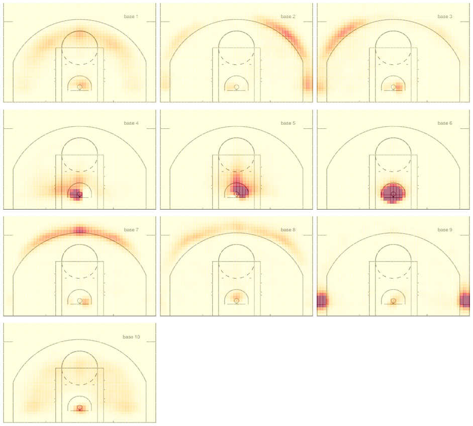
The central object is an intensity-dependent marked spatial point process. Shot locations are modeled by a non-homogeneous Poisson process with intensity $\lambda(s)$, and each binary make/miss mark is modeled by a logistic regression that includes $\lambda(s)$ as a covariate, $\logit(\theta(s)) = \xi\lambda(s)+Z(s)^\top\alpha$. Ten intensity bases built by nonnegative matrix factorization from prior-season shot data act as spatial covariates for $\lambda$, giving each location an interpretation as a shot type such as corner three or restricted-area two. MCMC draws from the joint posterior, with the Poisson integral approximated on a grid, and DIC and LPML compare the model with $\xi$ free against the model with $\xi=0$.

What would settle it

Re-fit the mark model with shot-clock time remaining included as a covariate for the same top-50 players; if the posterior mass of $\xi$ moves toward zero for a substantial share of the 40 players, or if DIC and LPML no longer favor $\xi\neq 0$ in most cases, the claimed positive intensity-accuracy association is partly an artifact of shot-clock confounding.

Watch

Extended reading notes

Core claim

The central claim is that shot intensity and shot accuracy are positively associated for a majority of elite NBA shooters, and that the association can be identified in a joint model rather than in two separate analyses. In the mark model $\logit(\theta(s_i)) = \xi\lambda(s_i) + Z(s_i)^\top\alpha$, the parameter $\xi$ is the quantity of interest: it says whether a player converts more often at locations where the fitted attempt intensity $\lambda$ is higher. For the four featured players, Durant, Harden, and James favored $\xi\neq 0$ by DIC and LPML, while Curry favored the intensity-independent model. Across the top 50 most frequent shooters, 40 favored $\xi\neq 0$ and all of those 40 had positive estimated $\xi$; the interaction between intensity and two-versus-three-point shot type was not significant in any of the 50, and for the 10 players preferring $\xi=0$, shot distance was significantly negative in every case. These results are the paper's central empirical discovery, supported by simulation studies showing that the MCMC estimator has near-nominal coverage.

Load-bearing premise

The load-bearing premise is that no unmeasured factor, especially shot-clock time remaining, inflates the estimated link between shot intensity and accuracy; the data do not include shot clock time, which the paper names as an important covariate missing from the mark model.

Editorial extensions

If this is right

For each of the 40 players with positive $\xi$, the coefficient provides a ranking of how efficiently that player converts his existing shot distribution into points at the spots he frequents.
Players whose estimated $\xi$ falls below the paper's elite average of about 1.02 are candidates for shot-selection improvement: shifting attempts toward their own high-intensity, high-accuracy zones should raise expected scoring.
The fitted intensity and mark surfaces combine into an expected-score map over the whole court, which remains meaningful even in locations where a player took few or no shots.
The absence of a significant intensity-by-shot-type interaction indicates the positive frequency-accuracy link does not differ between two-point and three-point attempts for these players.

Reading between the lines

Editorial extensions of the paper, not claims the author makes directly.

The authors do not test whether shot-clock pressure drives the association; adding it as a covariate is a natural check that could shrink $\xi$ for late-clock shooters.
A hierarchical version pooling all players with random effects would let $\xi$ vary by position and usage, testing whether the positive coupling is concentrated in high-usage stars rather than all shooters.
The same joint model could be run on play-by-play data with defender distance and shot-clock time, turning a descriptive association into a causal shot-selection diagnostic.

Share X Bluesky LinkedIn Reddit HN

Signed reviews

No signed human review yet.

Editorial analysis

A structured set of objections, weighed in public.

Desk editor's note, referee report, and a circularity audit.

Desk Editor's Note

read the letter

Good paper, with a real gap between the headline and the evidence. The methodological core—a Bayesian joint model of shot intensity and shot outcome for basketball—is new for this literature, and it's competently executed. The point process intensity is built from NMF basis shot types, the mark model includes the intensity as a covariate, and the MCMC estimation is validated with simulations showing small bias and coverage near 0.95. The four-player analyses are readable and the expected-score maps are a nice touch.

The main problem is the 40-of-50 majority claim. The paper says 40 of the top 50 shooters favored the intensity-dependent model by DIC and LPML, and all 40 estimated intensity coefficients were positive. But it never reports the magnitudes of the DIC/LPML differences or the credible intervals for those coefficients. The paper itself sets thresholds: DIC differences above 10 are substantial, 2–3 are weak; LPML differences above 4.5 are 'very strong'. The four-player table shows Durant called a 'clear advantage' with ΔDIC=8.6 and ΔLPML=4.2, both below those benchmarks. If a similar share of the 40 have weak differences, the 80% headline is overstated. Positive posterior means alone don't establish association; you need to know how many of the 40 have HPD intervals that exclude zero.

Minor issues: the reported results come from a second run after dropping insignificant covariates, which is post-hoc and makes the intervals a bit optimistic. The shot clock omission is acknowledged and is a genuine limitation, but not a fatal one.

The paper deserves a serious referee. The modeling and simulation are solid; the empirical claim needs more transparent reporting. I'd recommend sending it to review and asking for per-player summaries of model comparison and coefficient intervals.

Referee Report

4 major / 5 minor

Summary. The paper proposes a Bayesian marked spatial point process model for NBA shot charts, in which shot locations follow a non-homogeneous Poisson process with intensity covariates derived from nonnegative matrix factorization bases, and the binary shot-success mark is modeled by a logistic regression that includes the shot intensity as a covariate. Inference is performed with an MCMC algorithm implemented in NIMBLE, and model comparison is based on DIC and LPML. The estimation procedure is evaluated in simulation studies that report small bias and generally reasonable coverage. The method is applied to four named players and then to the top 50 most frequent shooters of the 2017–2018 NBA regular season, with the central empirical claim being that 40 of the 50 players favored the intensity-dependent mark model and that all 40 estimated intensity coefficients were positive. The fitted coefficients are also used as inputs for hierarchical clustering of the players.

Significance. If the central empirical finding holds, the paper offers a quantitative, data-driven measure of shot-selection efficiency and a practical joint modeling framework for marked spatial point processes with applications beyond sports. The work is methodologically constructive: it combines NMF basis construction, a Bayesian joint model, and model comparison criteria in a reproducible pipeline, and the simulation studies are reported in detail with tables of bias, standard deviation, and coverage. The paper also produces falsifiable empirical claims about top NBA shooters, which are of interest to the sports analytics community. However, the significance of the headline 40-of-50 result is currently limited by the lack of per-player evidence in the manuscript, the inconsistent application of the paper's own model-comparison thresholds, and the acknowledged omission of shot clock information that could confound the intensity-accuracy association.

major comments (4)

[Section 6.4 and Section 6.2] In addition, reporting only that the 40 estimated coefficients were positive is insufficient, because a positive posterior mean can occur even when the posterior mass overlaps zero substantially. The authors should report how many of the 40 players have HPD intervals for ξ that exclude zero, and ideally the posterior probabilities that ξ > 0.
[Section 6.2 and Table 1] The paper should also clarify whether a player is counted as favoring the intensity-dependent model when both DIC and LPML favor it, or when either criterion does, since the counting rule directly affects the reported 40-of-50 figure.
[Section 6.2 and Section 6.3] Additionally, the text in Section 6.2 says the reported results are from the second run, but Table 1 is presented before this caveat is explained in detail, which could mislead a reader who assumes the comparisons are from a single pre-specified model.
[Section 7 and Section 6.1] The manuscript should also avoid language in the abstract and introduction that overstates the finding as a general positive association without explicitly acknowledging this confounding risk at the point of the claim.

minor comments (5)

[Tables 3 and 4] The coverage summaries would be more interpretable if the Monte Carlo standard errors of the coverage rates were reported.
[Section 6.3] The sentence 'The might be due to his injury in that season and reduced time on court' in Section 6.3 contains a grammatical error ('The might be due') and appears to be an incomplete thought.
[Figure 4] The paper does not state what software was used for the hierarchical clustering beyond naming Ward's method and the R implementation; the specific function or package should be mentioned for reproducibility.
[General] The introduction and abstract state that the intensity-dependent model is preferred for 'a majority' of the top 50 shooters, while the introduction later says 'about 80%'; these statements should be consistent throughout the manuscript.
[Section 6.2] The text in Section 6.2 says that convergence was confirmed by trace plots, but does not report any quantitative convergence diagnostics, such as Gelman-Rubin statistics or effective sample sizes; adding these would strengthen the reproducibility of the MCMC results.

Circularity Check

0 steps flagged · score 1.0 of 10

No significant circularity: the intensity coefficient ξ is a fitted parameter in the joint likelihood, and the 40-of-50 finding is an empirical model comparison, not a prediction derived from its own inputs.

full rationale

The paper's load-bearing claim is that for a majority of top NBA shooters shot accuracy and shot intensity are positively associated. This is established by fitting the joint model in Eqs. (1)-(2), where ξ is an unknown regression coefficient estimated from the joint likelihood (3), and by comparing ξ = 0 against ξ ≠ 0 using DIC and LPML. Nothing in the model defines ξ in terms of the comparison outcome, and no fitted quantity is relabeled as a prediction; Section 6.4 simply reports fitted model comparisons and the signs of posterior means. The NMF shot-type bases follow Miller et al. (2014) and are constructed from historical 2016-2017 data, so they are not circular with respect to the 2017-2018 shot charts. The only self-citation is the LPML approximation for the intensity component in Eq. (8), attributed to Hu et al. (2019), which includes one of the present authors. That citation is not load-bearing for the main empirical conclusion: the detailed four-player analysis is supported by DIC as well as LPML, and the LPML formula is an approximation tool rather than the source of the estimated association. The shot-clock confounder acknowledged in Section 7 is a validity concern, not a circularity. Overall, the derivation chain is self-contained: the association is estimated from the data, not assumed, derived, or predicted from its own inputs.

Assumptions & free parameters 6 free parameters · 6 assumptions · 0 invented entities

The model's free parameters are the regression coefficients estimated from the data, with ξ being the central one. The axioms are the modeling choices: Poisson process for locations, log-linear intensity, logistic mark model, and the validity of NMF bases across seasons. No new physical or conceptual entities are introduced.

free parameters (6)

ξ (intensity coefficient in mark model) = Durant 1.237, Harden 1.291, James 0.632 (posterior means)
This is the central association parameter; it is estimated from the data, not derived or predicted.
λ0 (baseline intensity) = ranges 0.236 (Curry) to 0.423 (James)
Estimated from the shot attempts; scales the Poisson intensity.
β (10 basis intensity coefficients) = player-specific values in Table 2
Coefficients for the NMF shot-type bases in the log-intensity model.
α (mark model coefficients) = intercept and distance; e.g., Curry intercept -0.165, distance -0.270
Logistic regression coefficients for the mark model.
Number of NMF bases K = 10
Chosen by hand following Miller et al. (2014); not fitted from data, but affects the intensity covariate.
Kernel bandwidth for historical intensity maps = not specified
The paper uses kernel estimation (Section 6.1) but does not state the bandwidth; this affects the NMF basis construction.

assumptions (6)

domain assumption Shot locations follow a non-homogeneous Poisson process
Section 3.1 assumes N(A) is Poisson with mean λ(A); point interactions between shots are ignored.
domain assumption The log intensity is linear in the NMF basis covariates
Equation (1) sets λ(s) = λ0 exp(X^T(s) β); this functional form is assumed.
domain assumption The mark depends on intensity linearly on the logit scale
Equation (2) sets logit(θ(s)) = ξ λ(s) + Z^T(s) α; the linearity is assumed.
domain assumption The 10 NMF bases from historical data are valid for the current season
Section 6.1 constructs bases from 2016-2017 data and applies them to 2017-2018 shots.
domain assumption Marks are conditionally independent given intensity and covariates
Equation (3) factorizes the mark likelihood over shots; no spatial correlation in marks is modeled.
domain assumption Shot clock time remaining is absent and does not confound the association
Acknowledged in Section 7 as an important factor not available in the dataset.

how reviews work

0 comments

Cite this review

Pith. "Pith review of A Bayesian marked spatial point processes model for basketball shot chart." pith.science (2026). https://pith.science/paper/A7DRN2HR

@misc{pith2026190805745,
  author       = {Pith},
  title        = {Pith review of: A Bayesian marked spatial point processes model for basketball shot chart},
  year         = {2026},
  howpublished = {\url{https://pith.science/paper/A7DRN2HR}},
  note         = {Machine review of arXiv:1908.05745}
}

read the original abstract

The success rate of a basketball shot may be higher at locations where a player makes more shots. For a marked spatial point process, this means that the mark and the intensity are associated. We propose a Bayesian joint model for the mark and the intensity of marked point processes, where the intensity is incorporated in the mark model as a covariate. Inferences are done with a Markov chain Monte Carlo algorithm. Two Bayesian model comparison criteria, the Deviance Information Criterion and the Logarithm of the Pseudo-Marginal Likelihood, were used to assess the model. The performances of the proposed methods were examined in extensive simulation studies. The proposed methods were applied to the shot charts of four players (Curry, Harden, Durant, and James) in the 2017--2018 regular season of the National Basketball Association to analyze their shot intensity in the field and the field goal percentage in detail. Application to the top 50 most frequent shooters in the season suggests that the field goal percentage and the shot intensity are positively associated for a majority of the players. The fitted parameters were used as inputs in a secondary analysis to cluster the players into different groups.

Figures

Figures reproduced from arXiv: 1908.05745 by the authors.

**Figure 2.** Intensity matrix bases heat plots. left/right/center restricted area 2-points, basis 7 is top of key threes, basis 8 is center threes, basis 9 is corner threes, and basis 10 is mid-range twos. When used as covariates in modeling individual shot intensity, their coefficients characterize the shooting style of each player. The influence of intensity on shot accuracy might be different for different shot type. Players’… view at source ↗

**Figure 3.** Fitted shot intensity surfaces (upper) and expected score surfaces (lower) of Curry, [PITH_FULL_IMAGE:figures/full_fig_p013_3.png] view at source ↗

Figures from the paper (1 more)

**Figure 4.** Figure 4: Hierarchical clustering of 51 NBA players into 5 groups based on fitted coefficients [PITH_FULL_IMAGE:figures/full_fig_p015_4.png]

Discussion (0). Continue with ORCID to comment.

Reference graph

Works this paper leans on

32 extracted references · 31 canonical work pages

[1]

Alferink, L. A., T. S. Critchfield, J. L. Hitt, and W. J. Higgins (2009). Generality of the matching law as a descriptor of shot selection in basketball. Journal of Applied Behavior Analysis\/ 42\/ (3), 595--608

work page 2009
[2]

Turner, et al

Baddeley, A., R. Turner, et al. (2005). spatstat : A n R package for analyzing spatial point patterns. Journal of Statistical Software\/ 12\/ (6), 1--42

work page 2005
[3]

Banerjee, S., B. P. Carlin, and A. E. Gelfand (2014). Hierarchical Modeling and Analysis for Spatial Data . Chapman and Hall/ CRC

work page 2014
[4]

Baum, W. M. (1974). On two types of deviation from the matching law: Bias and undermatching. Journal of the Experimental Analysis of Behavior\/ 22\/ (1), 231--242

work page 1974
[5]

Shao, and J

Chen, M.-H., Q.-M. Shao, and J. G. Ibrahim (2000). M onte C arlo Methods in B ayesian Computation . Springer Science & Business Media

work page 2000
[6]

Cressie, N. (2015). Statistics for Spatial Data . John Wiley & Sons

2015
[7]

Turek, C

de Valpine, P., D. Turek, C. J. Paciorek, C. Anderson-Bergman, D. T. Lang, and R. Bodik (2017). Programming with models: Writing statistical algorithms for general model structures with NIMBLE . Journal of Computational and Graphical Statistics\/ 26\/ (2), 403--413

work page 2017
[8]

Diggle, P. J. (2013). Statistical Analysis of Spatial and Spatio-Temporal Point Patterns . Chapman and Hall/CRC

work page 2013

Show all 32 references

[9]

Miller, L

Franks, A., A. Miller, L. Bornn, K. Goldsberry, et al. (2015). Characterizing the spatial structure of defensive skill in professional basketball. The Annals of Applied Statistics\/ 9\/ (1), 94--121

2015
[10]

Gaujoux, R. and C. Seoighe (2010). A flexible R package for nonnegative matrix factorization. BMC Bioinformatics\/ 11\/ (1), 367

2010
[11]

Geisser, S. and W. F. Eddy (1979). A predictive approach to model selection. Journal of the American Statistical Association\/ 74\/ (365), 153--160

1979
[12]

Gelfand, A. E. and D. K. Dey (1994). B ayesian model choice: A symptotics and exact calculations. Journal of the Royal Statistical Society. Series B (Methodological)\/ 56\/ (3), 501--514

1994
[13]

Geyer, C. J. (1999). Likelihood inference for spatial point processes. In O. Barndorff-Nielsen, W. Kendall, and M. van Lieshout (Eds.), Stochastic Geometry: Likelihood and Computation , Volume 80, pp.\ 79--140. CRC Press

1999
[14]

Ho, L. P. and D. Stoyan (2008). Modelling marked point patterns by intensity-marked C ox processes. Statistics & Probability Letters\/ 78\/ (10), 1194--1199

2008
[15]

Huffer, and M.-H

Hu, G., F. Huffer, and M.-H. Chen (2019). New development of B ayesian variable selection criteria for spatial point process with applications. e-prints 1910.06870, arXiv

2019 arXiv
[16]

Kass, R. E. and A. E. Raftery (1995). Bayes factors. Journal of the american statistical association\/ 90\/ (430), 773--795

1995
[17]

Leininger, T. J., A. E. Gelfand, et al. (2017). B ayesian inference and model assessment for spatial point patterns using posterior predictive samples. Bayesian Analysis\/ 12\/ (1), 1--30

2017
[18]

Bornn, R

Miller, A., L. Bornn, R. Adams, and K. Goldsberry (2014). Factorized point process intensities: A spatial analysis of professional basketball. In Proceedings of the 31st International Conference on Machine Learning --- Volume 32 , ICML'14, pp.\ 235--243

2014
[19]

Miller, J. W. and M. T. Harrison (2018). Mixture models with a prior on the number of components. Journal of the American Statistical Association\/ 113\/ (521), 340--356

2018
[20]

M ller, J., A. R. Syversveen, and R. P. Waagepetersen (1998). Log gaussian C ox processes. Scandinavian Journal of Statistics\/ 25\/ (3), 451--482

1998
[21]

M ller, J. and R. P. Waagepetersen (2003). Statistical Inference and Simulation for Spatial Point Processes . Chapman and Hall/ CRC

2003
[22]

Goreaud, and J

Mrkvi c ka, T., F. Goreaud, and J. Chad uf (2011). Spatial prediction of the mark of a location-dependent marked point process: H ow the use of a parametric model may improve prediction. Kybernetika\/ 47\/ (5), 696--714

2011
[23]

Murtagh, F. and P. Legendre (2014). Ward’s hierarchical agglomerative clustering method: W hich algorithms implement W ard’s criterion? Journal of Classification\/ 31\/ (3), 274--295

2014
[24]

Reich, B. J., J. S. Hodges, B. P. Carlin, and A. M. Reich (2006). A spatial analysis of basketball shot chart data. The American Statistician\/ 60\/ (1), 3--12

2006
[25]

Skinner, B. (2012). The problem of shot selection in basketball. PloS One\/ 7\/ (1), e30776

2012
[26]

Skinner, B. and M. Goldman (2015). Optimal strategy in basketball. e-prints 1512.05652, arXiv

2015 arXiv
[27]

Spiegelhalter, D. J., N. G. Best, B. P. Carlin, and A. Van Der Linde (2002). B ayesian measures of model complexity and fit. Journal of the Royal Statistical Society: Series B (Statistical Methodology)\/ 64\/ (4), 583--639

2002
[28]

Staddon, J. (1978). Theory of behavioral power functions. Psychological Review\/ 85\/ (4), 305--320

1978
[29]

Vollmer, T. R. and J. Bourret (2000). An application of the matching law to evaluate the allocation of two- and three-point shots by college basketball players. Journal of Applied Behavior Analysis\/ 33\/ (2), 137--150

2000
[30]

Ward, Jr, J. H. (1963). Hierarchical grouping to optimize an objective function. Journal of the American Statistical Association\/ 58\/ (301), 236--244

1963
[31]

Zhang, D., M.-H. Chen, J. G. Ibrahim, M. E. Boye, and W. Shen (2017). B ayesian model assessment in joint modeling of longitudinal and survival data with applications to cancer clinical trials. Journal of Computational and Graphical Statistics\/ 26\/ (1), 121--133

2017
[32]

Lorenzo, M.-A

Zhang, S., A. Lorenzo, M.-A. G \'o mez, N. Mateus, B. Gon c alves, and J. Sampaio (2018). Clustering performances in the NBA according to players’ anthropometric attributes and playing experience. Journal of Sports Sciences\/ 36\/ (22), 2511--2520

2018

Pith tools

Reviewed August 14, 2026 · model on record in the stance chip above.

[1] [1]

Alferink, L. A., T. S. Critchfield, J. L. Hitt, and W. J. Higgins (2009). Generality of the matching law as a descriptor of shot selection in basketball. Journal of Applied Behavior Analysis\/ 42\/ (3), 595--608

work page 2009

[2] [2]

Turner, et al

Baddeley, A., R. Turner, et al. (2005). spatstat : A n R package for analyzing spatial point patterns. Journal of Statistical Software\/ 12\/ (6), 1--42

work page 2005

[3] [3]

Banerjee, S., B. P. Carlin, and A. E. Gelfand (2014). Hierarchical Modeling and Analysis for Spatial Data . Chapman and Hall/ CRC

work page 2014

[4] [4]

Baum, W. M. (1974). On two types of deviation from the matching law: Bias and undermatching. Journal of the Experimental Analysis of Behavior\/ 22\/ (1), 231--242

work page 1974

[5] [5]

Shao, and J

Chen, M.-H., Q.-M. Shao, and J. G. Ibrahim (2000). M onte C arlo Methods in B ayesian Computation . Springer Science & Business Media

work page 2000

[6] [6]

Cressie, N. (2015). Statistics for Spatial Data . John Wiley & Sons

2015

[7] [7]

Turek, C

de Valpine, P., D. Turek, C. J. Paciorek, C. Anderson-Bergman, D. T. Lang, and R. Bodik (2017). Programming with models: Writing statistical algorithms for general model structures with NIMBLE . Journal of Computational and Graphical Statistics\/ 26\/ (2), 403--413

work page 2017

[8] [8]

Diggle, P. J. (2013). Statistical Analysis of Spatial and Spatio-Temporal Point Patterns . Chapman and Hall/CRC

work page 2013