REVIEW 2 major objections 5 minor 31 references
Univalent Polynomials and Hubbard Trees
T0 review · 2 major / 5 minor · reviewed 2026-08-14 · deepseek-v4-flash
Pith's one-line read A single finite bi-angled tree uniquely encodes each extremal univalent polynomial, and the same trees classify all critically fixed anti-polynomials.
desk verdict Strong and likely correct classification, but the uniqueness half of Theorem A has a load-bearing gap around the combined quasiconformal map Ψ0. read the letter →
The pith
A machine-rendered reading of the paper's core claim, the machinery that carries it, and where it could break.
The reading
What carries the argument
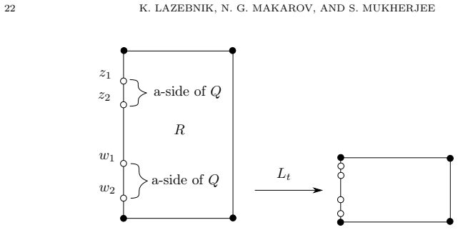
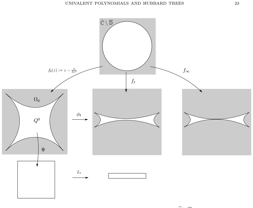
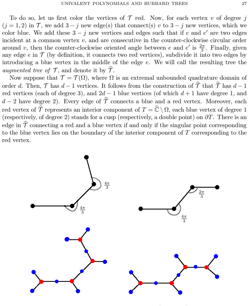
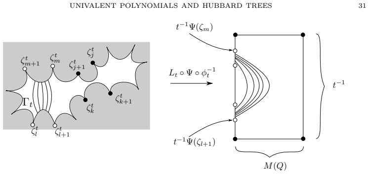
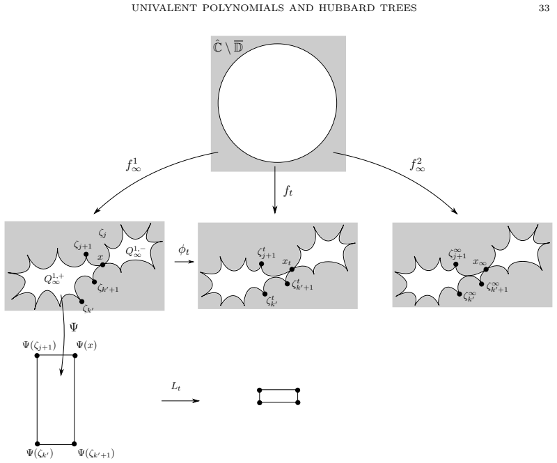
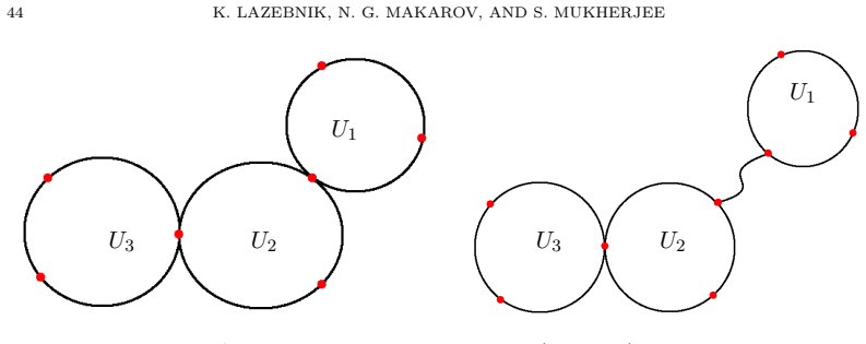
The central combinatorial object is the bi-angled tree: a tree with vertices of degree at most three, embedded so that all edges are straight segments meeting at angles $2\pi/3$ or $4\pi/3$, with an angle function encoding the cyclic order around each vertex. The load-bearing geometric construction is the pinching theorem: starting from the base map $f_0(z)=z-\frac{1}{d}z^d$ whose image is a hypocycloid, the paper uses Schwarz-reflection-invariant Beltrami coefficients, supported on preimages of a quadrilateral under the Schwarz reflection map, to stretch selected arcs and force specified pairs of arcs to meet, creating double points one at a time while preserving all other incidences. An augmented tree, obtained by inserting blue vertices into the bi-angled tree, lists which cusps and double points lie on which fundamental tiles and hence which arcs must be pinched. For uniqueness, the machinery is a pullback argument: a conformal map between two droplets with isomorphic trees is shown to be asymptotically linear at the singular points, extended to a global quasiconformal map, then lifted by iterates of the Schwarz reflections; the limit is conformal off a zero-area set and hence affine.
What would settle it
Take two extremal quadrature domains with isomorphic bi-angled trees and compute, in the coordinates that straighten each Schwarz reflection near infinity, the landing point of the fixed external ray corresponding to a shared cusp; if the two coordinates place that landing point at images that are not mapped to each other by the droplet homeomorphism, then no map with the required combined agreement can exist, and the uniqueness proof would need a different extension.
Extended reading notes
Core claim
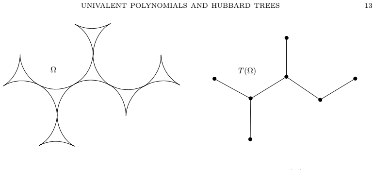
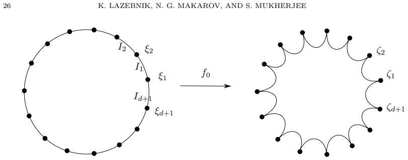
Every extremal $f\in\Sigma^*_d$—a rational map of degree $d+1$, univalent outside the closed unit disk, with $d+1$ cusps and $d-2$ double points on $f(\mathbb T)$—determines a droplet $\widehat{\mathbb C}\setminus f(\widehat{\mathbb C}\setminus \mathbb D)$, whose $d-1$ interior components are topological triangles. Treating each triangle as a vertex and joining two vertices when the triangles touch creates a bi-angled tree $\mathcal T(f)$. The paper proves two directions: first, every abstract bi-angled tree with $d-1$ vertices is realized by such an $f$ (surjectivity, via a pinching procedure), and second, two such $f$ realize isomorphic trees only if they differ by multiplication by a $(d+1)$-st root of unity (injectivity, via a quasiconformal pullback argument). Thus affine equivalence classes of extremal unbounded quadrature domains are in bijection with isomorphism classes of bi-angled trees. The same trees arise as the angled Hubbard trees of anti-holomorphic polynomials with $d-1$ distinct fixed critical points, and the paper invokes a realization theorem for angled trees to obtain the bijection with affine conjugacy classes of these anti-polynomials.
Load-bearing premise
Toward proving uniqueness, the argument needs a global quasiconformal map that simultaneously matches the prescribed homeomorphism between the two droplets and matches the coordinate straightening of the two Schwarz reflections near infinity and along the chosen fixed ray; the paper asserts such a combined extension exists, but the lemma it cites proves only that the droplet homeomorphism admits a quasiconformal extension.
Editorial extensions
If this is right
- Every bi-angled tree with $d-1$ vertices occurs in every degree; extremal Suffridge polynomials therefore exist in abundance rather than only by a convexity argument.
- Two extremal unbounded quadrature domains are affinely equivalent exactly when their bi-angled trees are isomorphic, so the geometric class is completely classified by finite trees.
- The classification extends to critically fixed anti-polynomials: affine conjugacy classes of degree-$d$ anti-polynomials with $d-1$ distinct fixed critical points are in bijection with bi-angled trees with $d-1$ vertices.
- In the bounded class $S^*_d$, the same methods give that extremal polynomials correspond to rooted binary trees with $d-2$ vertices, and the count is the Catalan number $\frac{1}{d-1}\binom{2d-4}{d-2}$.
- The shared tree invariant supplies a direct route from an extremal quadrature domain to a critically fixed anti-polynomial, making the dynamics of the Schwarz reflection map combinatorially accessible from the tree.
Reading between the lines
- The classification implies a count of affine equivalence classes of extremal unbounded quadrature domains: it is the number of bi-angled trees with $d-1$ vertices, which could be enumerated by a simple recurrence on plane trees.
- Because the proof realizes trees by pinching arcs, a natural testable extension is that non-extremal limits—where fewer double points are created—should be parameterized by the same trees with some edges left unpinched, i.e., bi-angled forests with marked active edges.
- The bijection between quadrature domains and critically fixed anti-polynomials suggests an explicit dictionary: properties of the Schwarz reflection tiling, such as external ray landing patterns, should be readable from the Hubbard tree's internal-ray angles, and conversely.
Signed reviews
Editorial analysis
A structured set of objections, weighed in public.
Referee Report
Summary. The paper studies external polynomials in Σ*_d whose image of the unit circle has the maximal number d−2 of double points (Suffridge polynomials), and proves a canonical bijection between such polynomials modulo the Z_{d+1}-action, isomorphism classes of bi-angled trees with d−1 vertices, and affine conjugacy classes of degree-d anti-polynomials with d−1 distinct fixed critical points (Crofoot–Sarason anti-polynomials). The proof combines a quasiconformal pinching construction for existence (Theorem 4.1), a pullback/quasiconformal rigidity argument for uniqueness (Theorem 5.1), and Poirier's classification of angled Hubbard trees for the anti-polynomial side. A parallel bijection for the class S*_d is used to enumerate extremal functions by Catalan numbers (Theorem B).
Significance. If the classification is correct, it is a substantial result: it completely describes all extremal unbounded quadrature domains in combinatorial terms and establishes a new bridge between quadrature domains and anti-holomorphic dynamics. The pinching technique for Σ*_d is a genuine methodological novelty, and Theorem B gives an elegant Catalan count that is likely to be of independent interest. The paper is also careful in several places: cusp types and tangency orders are proved from scratch (Propositions 2.9 and 2.10), the quasiconformal closure of the family is stated precisely (Proposition 3.3), and the use of Poirier's realization theorem is explicit. The main obstruction to accepting the paper as it stands is the incomplete proof of the combined quasiconformal extension in Theorem 5.1, which is load-bearing for the uniqueness half of the central classification.
major comments (2)
- [§5.1, proof of Theorem 5.1 (first paragraph after Lemma 5.4)] The proof defines a K-quasiconformal map Ψ0 that agrees with Ψ on the droplet ~T and with τ∘τ~^{-1} on U∪R0(~σ), and states: 'The existence of such a map is guaranteed by Lemma 5.4.' Lemma 5.4, however, only establishes a quasiconformal extension of Ψ to the sphere; it says nothing about matching the Böttcher conjugacy on the invariant neighborhood U or along the fixed ray R0(~σ), and no interpolation across the region between U and the droplet is constructed. This is not a cosmetic omission: the subsequent lifts Ψ1,Ψ2,... and the normalization Ψ1(~ζ0)=ζ0 depend on having a single K-quasiconformal map that simultaneously realizes both prescribed behaviors. Without such a map, the identity (32), the statement Ψ1=Ψ0 on U, and the conclusion that the limiting Ψ∞ is conformal (hence affine) are unsupported. A separate gluing/interpolation lemma is needed that starts from Lemma 5.4 and the asymptotic linearity of Lemma 5.3 and produces Ψ0 with the stated boundary data and uniformly bounded dilatation; the manuscript should also specify how large U is and how the fixed ray is treated in the interpolation.
- [§4.2, proof of Theorem 4.1 (after Proposition 4.13)] The recursive pinching construction is not written for a general bi-angled tree. After the second step, the proof says 'subsequent steps are completely analogous' and stops. Since the construction is recursive over the set S_T of pinched pairs, one needs an induction statement that after each pinching step (i) the previously created double points persist in the limit, (ii) no new intersections are created outside the prescribed pairs, and (iii) the quadrilateral chosen for the next pair is admissible. The second step already requires a separate treatment when one of the chosen arcs has an endpoint at the existing double point; later steps may involve several pre-existing double points, and the curvature/modulus arguments in Proposition 4.13 would need to be re-run in that generality. This is a completeness gap in the existence half of Theorem A. The method is plausible and the gap appears repairable, but as written the proof relies on an unstated induction.
minor comments (5)
- [§5.1, Böttcher coordinate paragraph] The text says the conformal isomorphism τ conjugates z^d to σ, but σ is anti-meromorphic; the standard statement is a conjugacy to \bar z^d (or, after passing to σ^2, to z^{d^2}). Please correct the statement or the convention.
- [Lemma 5.4, proof] The sentence 'in fact, we have showed that \hatΨ : T→T is C1' is stronger than what is proved: Lemma 5.3 gives asymptotic linearity at the singular points and conformality away from them, which implies local quasisymmetry but not global C1 regularity. Please rephrase.
- [Lemma 5.4 and Section 5 generally] The symbol T is used both for the droplet \hat C\\Ω (Definition 2.15) and for the unit circle in the lifting diagram in Lemma 5.4. This notational clash makes the proof harder to follow; use \mathbb T or a different letter for the unit circle.
- [Definition 2.19] The phrase 'allowing for edges to decrease in length so as to avoid self-intersection' describes the recursive construction of the bi-angled tree informally. Since the bi-angled tree is a central invariant, a formal statement that this procedure terminates and produces an embedded tree would improve the exposition.
- [Table 1] The last three Suffridge polynomials in Table 1 are numerical approximations; it would be helpful to state the precision or to indicate the sense in which they are normalized.
Circularity Check
No circularity: the bi-angled tree classification is derived from independent existence and uniqueness arguments; cited prior work supplies supporting lemmas rather than restating the conclusion.
full rationale
The derivation chain is self-contained in the relevant sense. The map from Suffridge polynomials to bi-angled trees is defined geometrically (Definition 2.19), and the converse existence (Theorem 4.1) is proved by an explicit quasiconformal pinching construction starting from f0(z)=z−1/d z^d; no parameter is fitted from the target classification. Uniqueness (Theorem 5.1) is attempted through a pullback argument, and its auxiliary facts—constant conformal curvature, absence of wandering components, cusp/double-point asymptotics—are cited from prior external work [LM14, LLMM18a, LLMM18b], not from the conclusion of Theorem A. The correspondence with CS anti-polynomials (Theorem 6.6) rests on Poirier's external realization and uniqueness theorem for angled Hubbard trees; the present-paper input is the observation that the identity angled tree map with local degree 2 makes a bi-angled tree a CS Hubbard tree. The skeptical issue in Theorem 5.1—the unsupported simultaneous quasiconformal extension Ψ0 matching both Ψ and the Böttcher conjugacy—is a potential correctness gap, not a circular reduction: Lemma 5.4 is not claimed to define Ψ0 by construction, and the missing interpolation is not an equation equating the theorem's output with its input. Self-citations such as [LMM20, §4] for landing of fixed external rays are peripheral supporting facts, not the classification content, and do not make the central claim equivalent to its assumptions.
Assumptions & free parameters
assumptions (7)
- standard math Quasiconformal deformation theory and the measurable Riemann mapping theorem (used to define φt in Propositions 4.3, 4.9, 4.12).
- standard math Sullivan's non-wandering theorem adaptation (used in Proposition 3.4 to rule out wandering Fatou components).
- domain assumption Poirier's realization and uniqueness theorem for angled Hubbard trees of postcritically finite anti-polynomials (used in Proposition 6.5 and Theorem 6.6).
- domain assumption Constant conformal curvature of f(T) at non-cusp points for f in Σ*_d (Principle 1, from [LM14, Corollary 2.8]).
- domain assumption Khavinson-Swiatek upper bound of 3d−2 fixed points for harmonic polynomials (Theorem 2.21, from [KS03]).
- standard math Warschawski's asymptotic formulas for conformal maps of curvilinear strips (used in Lemma 5.3).
- standard math Ahlfors-Beurling extension theorem and removability of analytic arcs and measure-zero sets (used in Lemmas 5.4 and the proof of Theorem 5.1).
Cite this review
Pith. "Pith review of Univalent Polynomials and Hubbard Trees." pith.science (2026). https://pith.science/paper/WKIWJTEY
@misc{pith2026190805813,
  author       = {Pith},
  title        = {Pith review of: Univalent Polynomials and Hubbard Trees},
  year         = {2026},
  howpublished = {\url{https://pith.science/paper/WKIWJTEY}},
  note         = {Machine review of arXiv:1908.05813}
}
abstract
We study rational functions $f$ of degree $d+1$ such that $f$ is univalent in the exterior unit disc, and the image of the unit circle under $f$ has the maximal number of cusps ($d+1$) and double points $(d-2)$. We introduce a bi-angled tree associated to any such $f$. It is proven that any bi-angled tree is realizable by such an $f$, and moreover, $f$ is essentially uniquely determined by its associated bi-angled tree. This combinatorial classification is used to show that such $f$ are in natural 1:1 correspondence with anti-holomorphic polynomials of degree $d$ with $d-1$ distinct, fixed critical points (classified by their Hubbard trees).
Figures
Figures from the paper (12 more)



Reference graph
Works this paper leans on
-
[1]
L. V. Ahlfors. Lectures on Quasiconformal Mappings (Second Edition) , volume 38 of University Lecture Series . American Mathematical Society, Providence, R.I., 2006
work page 2006
-
[2]
D. Aharonov and H. S. Shapiro. Domains on which analytic functions satisfy quadrature identities. J. Analyse Math. , 30:39--73, 1976
work page 1976
-
[3]
B. Branner and N. Fagella. Quasiconformal surgery in holomorphic dynamics , volume 141 of Cambridge Studies in Advanced Mathematics . Cambridge University Press, 2014
work page 2014
-
[4]
D. Bshouty and A. Lyzzaik. On C rofoot- S arason's conjecture for harmonic polynomials. Comput. Methods Funct. Theory , 4(1):35--41, 2004
work page 2004
-
[5]
D. A. Brannan. Coefficient regions for univalent polynomials of small degree. Mathematika , 14:165--169, 1967
work page 1967
-
[6]
X. Buff. Virtually repelling fixed points. Publicacions Matem \`a tiques , 47:195--209, 2003
work page 2003
-
[7]
L. Carleson and T. W. Gamelin. Complex Dynamics . Springer, Berlin, 1993
work page 1993
-
[8]
V. F. Cowling and W. C. Royster. Domains of variability for univalent polynomials. Proc. Amer. Math. Soc. , 19:767--772, 1968
work page 1968
Show all 31 references
-
[9]
Douady and J
A. Douady and J. H. Hubbard. \'E tude dynamique des polyn\^omes complexes . Soci \'e t \'e M ath \'e matique de F rance, 2007
2007
-
[10]
Peter L. Duren. Univalent functions , volume 259 of Grundlehren der Mathematischen Wissenschaften [Fundamental Principles of Mathematical Sciences] . Springer-Verlag, New York, 1983
1983
-
[11]
L. Geyer. Sharp bounds for the valence of certain harmonic polynomials. Proc. Amer. Math. Soc. , 136:549--555, 2008
2008
-
[12]
K \"o ssler
M. K \"o ssler. Simple polynomials. Czechoslovak Math. J. , 1(76):5--15, 1951
1951
-
[13]
Khavinson and G
D. Khavinson and G. Swiatek. On the number of zeros of certain harmonic polynomials. Proc. Amer. Math. Soc. , 131:409--414, 2003
2003
-
[14]
S. V. F. Levy. Critically Finite Rational Maps (Thurston) . ProQuest LLC, Ann Arbor, MI, 1985. Thesis (Ph.D.)--Princeton University
1985
-
[15]
S.-Y. Lee, A. Lerario, and E. Lundberg. Remarks on W ilmshurst's theorem. Indiana University Mathematics Journal , 64(4):1153--1167, 2015
2015
-
[16]
S.-Y. Lee, M. Lyubich, N. G. Makarov, and S. Mukherjee. Dynamics of S chwarz reflections: The mating phenomena. https://arxiv.org/abs/1811.04979v2, 2018
2018 arXiv
-
[17]
S.-Y. Lee, M. Lyubich, N. G. Makarov, and S. Mukherjee. S chwarz reflections and the T ricorn. https://arxiv.org/abs/1812.01573v1, 2018
2018 arXiv
-
[18]
Lee and N
S.-Y. Lee and N. Makarov . Sharpness of connectivity bounds for quadrature domains . https://arxiv.org/abs/1411.3415, 2014
2014 arXiv
-
[19]
Lee and N
S.-Y. Lee and N. G. Makarov. Topology of quadrature domains. J. Amer. Math. Soc. , 29(2):333--369, 2016
2016
-
[20]
Lazebnik, N
K. Lazebnik, N. G. Makarov, and S. Mukherjee. Bers slices in families of univalent maps. https://arxiv.org/abs/2007.02429v2, 2020
2007 arXiv
-
[21]
Lehto and K
O. Lehto and K. I. Virtanen. Quasiconformal mappings in the plane . Springer-Verlag, New York-Heidelberg, second edition, 1973. Translated from the German by K. W. Lucas, Die Grundlehren der mathematischen Wissenschaften, Band 126
1973
-
[22]
M. Yu. Lyubich. On typical behavior of the trajectories of a rational mapping of the sphere. Dokl. Akad. Nauk SSSR , 268:22--25, 1983
1983
-
[23]
C. Michel. Eine B emerkung zu schlichten P olynomen. Bull. Acad. Polon. Sci. S\' e r. Sci. Math. Astronom. Phys. , 18:513--519, 1970
1970
-
[24]
J. Milnor. Dynamics in one complex variable , volume 160 of Annals of Mathematics Studies . Princeton University Press, Princeton, NJ, third edition, 2006
2006
-
[25]
A. Poirier. Hubbard forests. Ergodic Theory and Dynamical systems , 33:303--317, 2013
2013
-
[26]
D. Sarason. written communication. Feb. 1999, Oct. 2000
1999
-
[27]
T. J. Suffridge. On univalent polynomials. J. London Math. Soc. , 44:496--504, 1969
1969
-
[28]
T. J. Suffridge. Extreme points in a class of polynomials having univalent sequential limits. Trans. Amer. Math. Soc. , 163:225--237, 1972
1972
-
[29]
Sullivan
D. Sullivan. Quasiconformal homeomorphisms and dynamics I . solution of the F atou- J ulia problem on wandering domains. Annals of Mathematics , 122(2):401--418, 1985
1985
-
[30]
S. E. Warschawski. On conformal mapping of infinite strips. Transactions of the American Mathematical Society , 51(2):280--335, 1942
1942
-
[31]
A. S. Wilmshurst. The valence of harmonic polynomials. Proc. Amer. Math. Soc. , 126(7):2077--2081, 1998
1998
Reviewed August 14, 2026 · model on record in the stance chip above.
Discussion (0). Continue with ORCID to comment.