Linear Stochastic Dividend Model

Sander Willems

REVIEW 2 major objections 5 minor 12 references

Linear Stochastic Dividend Model

T0 review · 2 major / 5 minor · reviewed 2026-08-14 · deepseek-v4-flash

Challenge this review Re-run · record.json Download PDF Read on arXiv ↗ Review JSON

Pith's one-line read Capping dividends by a stock fraction yields closed-form futures

desk verdict A genuinely useful single-factor dividend model with closed-form futures prices, but the uniqueness-in-law proof needs a patch before the paper is watertight. read the letter →

arxiv 1908.05850 v2 pith:6A3PJNHJ submitted 2019-08-16 q-fin.MF q-fin.CPq-fin.PR

Sander Willems This is my paper · ORCID

classification q-fin.MFq-fin.CPq-fin.PR MSC 91G2060J6060H10

keywords stochasticdividendmodelpolynomialdiffusionfuturesmaximumentropyapproximationstockoptionpricingyieldno-bubbleconditionlinearfactor

verification ladder T0 review T1 audit T2 compute T3 formal

The pith

A machine-rendered reading of the paper's core claim, the machinery that carries it, and where it could break.

The reading

This paper proposes a way to directly model the dividend rate of a stock, rather than the dividend yield, while keeping the stock price positive. The trick is to bound the dividend rate by a constant fraction of the stock price, so dividends vanish as the stock approaches zero. The resulting diffusion is polynomial, giving closed-form prices for stock and dividend futures and accurate maximum-entropy approximations for options. A calibration to Euro Stoxx 50 data shows the single-factor version fits the dividend futures term structure within about 2% and matches at-the-money index and dividend option implied volatilities.

What carries the argument

The central object is the state space $E$ with the upper bound $D_t \le a X_t$, which couples the dividend rate to the stock price so dividends go to zero with the price. Carrying the argument is the linear drift structure of $(X_t, Y_t)$: the generator maps polynomials to polynomials ($G\mathrm{Pol}_n \subseteq \mathrm{Pol}_n$), which makes $(C_t, X_t, Y_t)$ a polynomial diffusion and yields the moment formula (12). The no-bubble result uses the linear ODE system for discounted expectations plus Barbalat's lemma to show $\lim_{T\to\infty} E_t[e^{-r(T-t)} X_T] = 0$.

What would settle it

Evaluate the diffusion coefficient of $Y_t/X_t$ from the SDEs (2)-(3) near the boundary $X_t = 0$; if it behaves like $1/\sqrt{X_t}$ and is not uniformly bounded on the state space, then the cited uniqueness theorem (Ikeda–Watanabe Theorem IV.3.3) does not apply and the model's pricing formulas are not attached to a single well-defined solution.

Watch

Extended reading notes

Core claim

The paper claims that the SDE pair (2)-(3) defines a unique solution in $E = \{x>0, y\ge 0, 1^\top y \le ax\}$ under parameter conditions (4)-(5), with the stock price strictly positive and the dividend rate nonnegative; that the augmented process $(C_t, X_t, Y_t)$ is a polynomial diffusion so all conditional moments are available in closed form through the matrix-exponential formula $E_t[H_n(C_T,X_T,Y_T)] = e^{G_n(T-t)} H_n(C_t,X_t,Y_t)$; and that, when $1^\top b > 0$, the stock price equals the present value of all future dividends, so the model contains no bubble. On this basis futures prices are explicit and option prices are approximated by matching moments with the maximum-entropy density.

Load-bearing premise

The load-bearing step is the claim that $(\log X_t, Y_t/X_t)$ has uniformly bounded drift and diffusion coefficients; the diffusion of $Y_t/X_t$ near $X_t = 0$ involves a $1/\sqrt{X_t}$ factor, so that boundedness is not established and uniqueness in law is unsupported as written.

Editorial extensions

If this is right

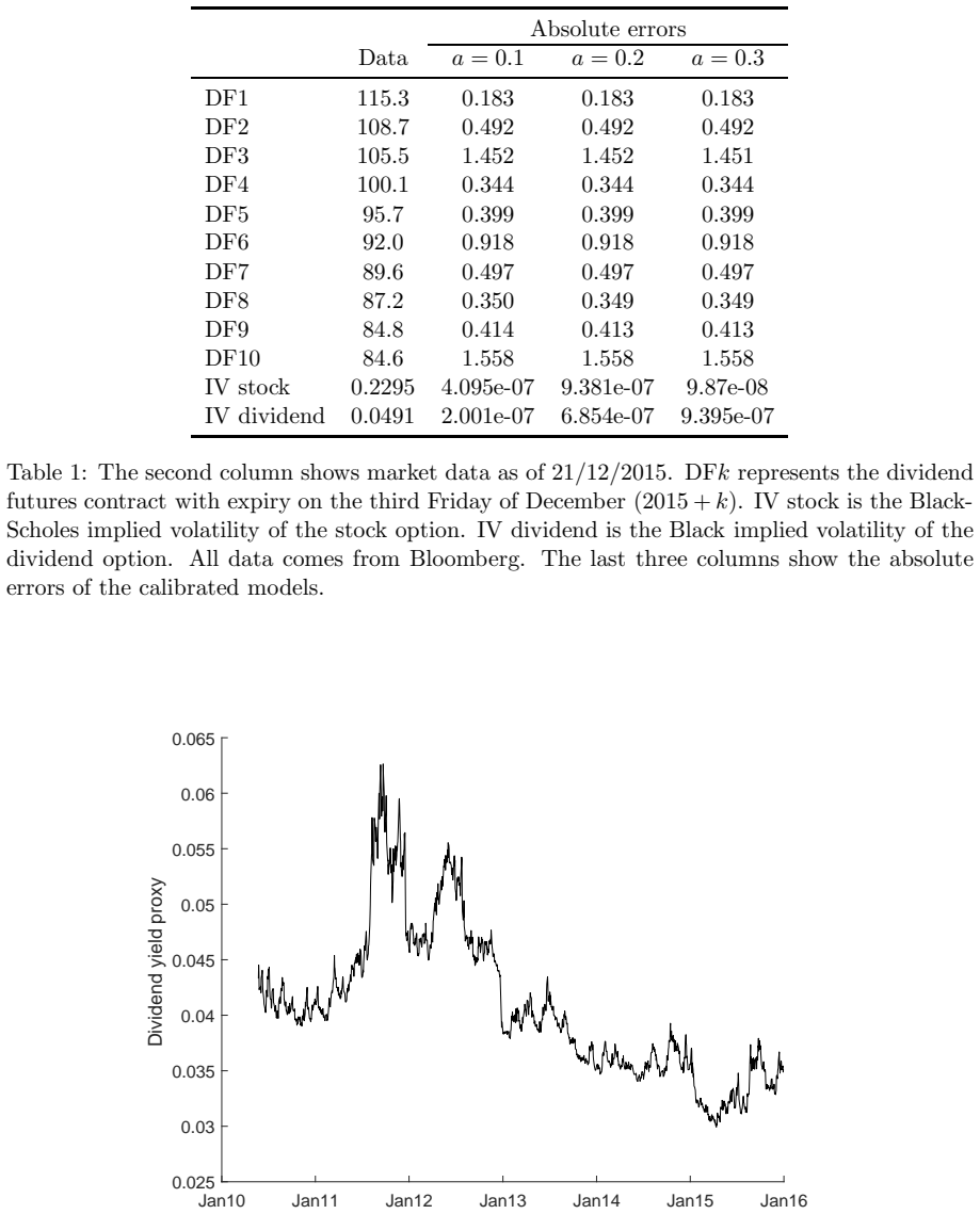
Stock and dividend futures prices are available in closed form, and the volatility parameters $\sigma$ and $\nu$ do not enter futures prices, so they can be calibrated separately to derivatives.
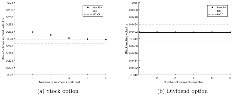
Stock and dividend option prices can be approximated by a maximum-entropy density matched to the first $N$ moments, with $N$ as small as four for stock options and two for dividend options in the numerical study.
Under the parameter condition $1^\top b > 0$, the stock price is equal to the present value of future dividends, ruling out a price bubble in the model.
The single-factor specification reproduces the empirical pattern of low volatility in short-dated dividend futures and high volatility in long-dated ones and the stock.
Adding jumps in the stock price preserves the polynomial property, so the same moment machinery extends to jump-diffusion versions.

Reading between the lines

Editorial extensions of the paper, not claims the author makes directly.

If the polynomial structure is the point, the same state-space-bound trick could be applied to other linear factor models, such as in credit or commodity markets, where a positive non-traded quantity must track a traded underlying.
The no-bubble condition $1^\top b > 0$ is testable empirically: if the model is right, long-dated dividend futures should move one-for-one with the stock index, while short-dated ones should have their own dynamics.
The moment-matching approach could be extended to more complex exotics, such as Asian options on cumulative dividends, because all mixed moments of $(C_T, X_T)$ are known in closed form.
A potential route to discrete dividends is to define $D_t$ as an intensity and make actual payments a point process; the polynomial property would survive if the jump intensity is affine in the factors.

Share X Bluesky LinkedIn Reddit HN

Signed reviews

No signed human review yet.

Editorial analysis

A structured set of objections, weighed in public.

Desk editor's note, referee report, and a circularity audit.

Desk Editor's Note

read the letter

The paper is worth a look if you care about dividend derivatives. It specifies the dividend rate as a linear function of a polynomial diffusion, with the stock price as the upper-bound process aX_t. The single-factor version is neat: D_t mean-reverts around a fraction of X_t, and because of the cap, X_t stays positive. You get closed-form futures prices and a max-entropy moment-matching approximation for options.

What is genuinely good: the model is a sensible special case of the author's earlier polynomial framework, and the no-bubble result (Proposition 2.3) is nicely proved via Barbalat. The generator computations are clean. The numerical section is honest about what it is—a calibration demonstration, not a horse race. The fit to the ten dividend futures is decent, and the option approximation converges quickly in their Monte Carlo comparison.

Soft spots, in proportion. The uniqueness-in-law proof in Appendix A.1 is incomplete. The claim that (log X, Y/X) has uniformly bounded coefficients is actually true—the reader's concern about a 1/sqrt(X) term is a red herring, since Z=Y/X lives in a compact simplex and the square-root terms are bounded. But boundedness alone does not make Ikeda–Watanabe IV.3.3 apply to a degenerate multi-dimensional SDE with non-Lipschitz coefficients. You need more: a Yamada–Watanabe argument, or a result from the polynomial diffusion theory (Filipović–Larsson). This matters because without uniqueness in law, the expectation formulas in Section 3 are not pinned to a single model. The fix is probably routine, but the text does not contain it.

Second, the max-entropy density is asserted as the unique solution; existence of the Lagrange multipliers is not addressed. In practice it works, but a rigorous reader will want a citation or a note.

Third, the calibration fits two ATM options with free sigma and nu, so the perfect match is not evidence of predictive power. They do not overclaim—it is a proof-of-concept.

Would I referee it? Yes. It is a clean, useful paper with one gap that can be patched. Send it back for a revision, don't desk reject.

Referee Report

2 major / 5 minor

Summary. The paper introduces a continuous-time model for jointly pricing stock and dividend derivatives. The dividend rate D_t is a linear function of a factor process Y_t, and the stock price X_t is specified so that it remains positive while the dividend yield is bounded by a constant a. The dynamics form a polynomial diffusion, yielding closed-form conditional moments, futures prices, and maximum-entropy option approximations. A single-factor version is calibrated to Euro Stoxx 50 dividend futures and ATM options with small errors. The paper also proves absence of price bubbles under the condition 1^T b > 0 and extends the model with jumps in the stock price.

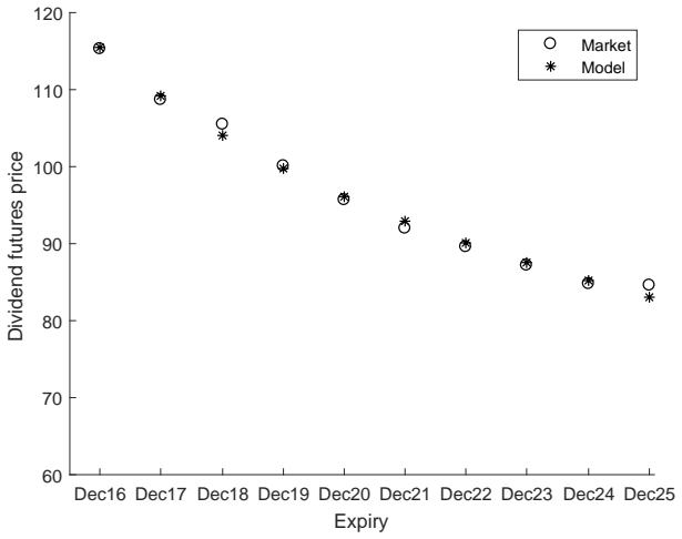
Significance. If the well-posedness gap identified below is fixed, this is a useful and tractable addition to the dividend-derivative literature. The main strengths are the closed-form linear derivative prices, the moment-based approximation for options, and the explicit no-bubble result showing that the stock price equals the present value of future dividends. The calibration exercise is transparent and demonstrates a good fit to a ten-maturity dividend futures curve plus two at-the-money options. The paper also gives self-contained computations of the generator and moment formula, and the jump extension preserves the polynomial structure.

major comments (2)

[Appendix A.1 (Proof of Proposition 2.1)] The uniqueness-in-law proof is incomplete. The final paragraph states that (log X_t, Y_t/X_t) has a uniformly bounded drift and diffusion function, so uniqueness follows from Ikeda–Watanabe (1981, Theorem IV.3.3). The boundedness assertion is correct: Y_t/X_t lies in the compact simplex {z >= 0, 1^T z <= a}, and the diffusion coefficient of the transformed process contains no 1/sqrt(X_t) singularity. The problem is that boundedness alone is not a sufficient condition for weak uniqueness of a degenerate multi-dimensional SDE, and the hypotheses of Theorem IV.3.3 are neither stated nor verified. In particular, the diagonal diffusion coefficient nu_k sqrt(z_k (1 - 1^T z / a)) is not Lipschitz at z_k = 0, so a Lipschitz-based uniqueness theorem does not apply. Because the moment formula (12) and the futures pricing formulas (13)-(14) require expectations under a unique risk-neutral measure, this gap is load-bearing. A fix is likely available from the polynomial-diffusion well-posedness results of Filipović–Larsson (2016) or a Yamada–Watanabe argument for the diagonal coefficients, but the current text does not supply it.
[Appendix A.1 (Proof of Proposition 2.1, existence step)] The existence step cites Ikeda–Watanabe Theorem IV.2.4 for an R^{1+d}-valued solution because the drift and dispersion coefficients satisfy a linear growth condition. However, the dispersion coefficient contains sqrt(x - 1^T y / a), which is not defined when x < 1^T y / a. To apply a global existence theorem, the coefficients must be extended from E to all of R^{1+d} in a way that preserves linear growth and continuity, and the extended system must be shown to have a solution that does not leave E before it is shown that it cannot leave E. As written, the existence argument is incomplete. This is a technical but fixable gap that should be addressed in the revision.

minor comments (5)

[Introduction and Section 2] There are repeated words: 'of of' in the Introduction and 'linear hypercube model model' in Section 2.
[Appendix A.1, equation (19)] The index in the minimum is written 'min_{l≠d}' and should be 'min_{l≠k}'.
[Section 3.3] The maximum-entropy method should briefly discuss the existence and uniqueness of the exponential-form density for a given moment vector; not every moment sequence lies in the interior of the feasible set, and the numerical solver's behavior is not described.
[Section 5, jump generator] In the expression for the jump generator, the term '− f − (x − 1^T y/a)z f_x' appears to be missing the second function evaluation; it should read 'f(c, x + (x - 1^T y/a)z, y) - f(c,x,y) - (x - 1^T y/a)z f_x'.
[Appendix A.2] 'To proof that' should be 'To prove that'.

Circularity Check

0 steps flagged · score 2.0 of 10

No significant circularity: pricing formulas are derived from the specified SDEs; the one self-citation is methodological, and the perfect option fit is an acknowledged in-sample calibration.

full rationale

The derivation chain is self-contained. Proposition 2.1 imposes explicit parameter conditions (4)-(7) and sketches existence and boundary non-attainment using the generator and comparison arguments; Section 3 computes the generator G directly from the stated dynamics (2)-(3) and obtains the moment formula (12) and futures prices (13)-(14) as algebraic consequences, not as model inputs. Proposition 2.3 derives the no-bubble property from the linear ODE for conditional expectations and Barbalat's lemma; it does not assume equation (8). The numerical section calibrates b, beta, sigma, nu1, and D0 to market data; the 'perfect' match of the two at-the-money option implied volatilities is explicitly explained as a consequence of sigma and nu1 being free once dividend futures are matched, so it is an in-sample fit rather than a predicted out-of-sample quantity. The citations to Filipovic-Willems (2018) and Filipovic-Larsson (2016) are used for the max-entropy approximation scheme and polynomial-diffusion technology; the present paper verifies its own polynomial invariance ('It is easily verified that GPol_n subset Pol_n') and supplies its own boundary and no-bubble proofs. The cited framework is external and not load-bearing in the sense of assuming the target results. The only notable technical weakness is in Appendix A.1: the claim that uniform boundedness of the drift and diffusion of (log X_t, Y_t/X_t) suffices for uniqueness in law via Ikeda-Watanabe Theorem IV.3.3 is not substantiated by a statement and verification of that theorem's hypotheses, and the square-root coefficients are non-Lipschitz near zero. That is a correctness gap in an external theorem application, not a circularity, because it does not assume the uniqueness conclusion or any pricing formula.

Assumptions & free parameters 7 free parameters · 5 assumptions · 1 invented entities

The central pricing formulas rest on polynomial process moment computations from prior literature, on the boundary-invariance argument, and on an assumed maximum-entropy solution. The calibration parameters are fitted to market data, and the only introduced modeling entity is the latent dividend factor process.

free parameters (7)

a = 0.1, 0.2, 0.3
Upper bound for the dividend yield, chosen by hand in the calibration; it constrains the admissible values of b and beta.
r = 0.01
Short rate fixed by hand to a representative level for the calibration date.
b = 0.0103
Calibrated to Euro Stoxx 50 dividend futures; identical across the three values of a.
beta = -0.3440
Calibrated to Euro Stoxx 50 dividend futures; nearly identical across the three values of a.
sigma = 0.3621, 0.2813, 0.2614
Calibrated to the at-the-money stock option and dividend option; the fitted value decreases as a increases.
nu1 = 0.0220, 0.0194, 0.0187
Calibrated to the at-the-money stock option and dividend option; the fitted value decreases as a increases.
D0 = 0.0371
Initial dividend rate, calibrated; identical across the three values of a.

assumptions (5)

standard math Linear growth of drift and dispersion coefficients guarantees weak existence of an R^{1+d}-valued solution to the SDE.
Invoked in the proof of Proposition 2.1 via Ikeda and Watanabe (1981), Theorem IV.2.4.
standard math Polynomial diffusion theory, including Theorem 5.7 of Filipovic and Larsson (2016), provides boundary non-attainment criteria and closed-form moment formulas.
Used in the proofs of Proposition 2.1 and the moment formula (12) without restating the full theory.
ad hoc to paper The maximum-entropy problem with moment constraints has a unique solution of exponential form.
Section 3.3 asserts the exponential density f^(N)(x)=exp(-sum lambda_n x^n) is the unique solution to (16), but existence, integrability, and uniqueness of the constrained maximizer are not proved.
domain assumption Continuously paid dividends are an acceptable approximation for index dividend derivatives.
Stated in the introduction as a footnote; most liquid dividend derivatives reference index dividends, and continuous payments are treated as acceptable.
ad hoc to paper The transformed process (log X_t, Y_t/X_t) has uniformly bounded drift and diffusion.
Asserted in the last paragraph of Appendix A.1 to prove uniqueness in law. The diffusion coefficient of Y_t/X_t is not uniformly bounded near X_t=0, so this assertion is false as written.

invented entities (1)

Latent factor process Y_t
purpose: Drives the stochastic dividend rate D_t = 1^T Y_t, with Y_t constrained so that D_t is nonnegative and bounded above by a X_t.
Y_t is unobservable and is a modeling construct. It has no independent empirical handle, although the model's option prices are testable.

how reviews work

0 comments

Cite this review

Pith. "Pith review of Linear Stochastic Dividend Model." pith.science (2026). https://pith.science/paper/6A3PJNHJ

@misc{pith2026190805850,
  author       = {Pith},
  title        = {Pith review of: Linear Stochastic Dividend Model},
  year         = {2026},
  howpublished = {\url{https://pith.science/paper/6A3PJNHJ}},
  note         = {Machine review of arXiv:1908.05850}
}

read the original abstract

In this paper we propose a new model for pricing stock and dividend derivatives. We jointly specify dynamics for the stock price and the dividend rate such that the stock price is positive and the dividend rate non-negative. In its simplest form, the model features a dividend rate that is mean-reverting around a constant fraction of the stock price. The advantage of directly specifying dynamics for the dividend rate, as opposed to the more common approach of modeling the dividend yield, is that it is easier to keep the distribution of cumulative dividends tractable. The model is non-affine but does belong to the more general class of polynomial processes, which allows us to compute all conditional moments of the stock price and the cumulative dividends explicitly. In particular, we have closed-form expressions for the prices of stock and dividend futures. Prices of stock and dividend options are accurately approximated using a moment matching technique based on the principle of maximal entropy.

Figures

Figures reproduced from arXiv: 1908.05850 by the authors.

**Figure 2.** Market prices and model implied prices of dividend [PITH_FULL_IMAGE:figures/full_fig_p012_2.png] view at source ↗

**Figure 3.** Simulation the dividend yield process δt over ten years with daily discretization. The model parameters are those in [PITH_FULL_IMAGE:figures/full_fig_p012_3.png] view at source ↗

Figures from the paper (1 more)

**Figure 4.** Figure 4: Option price approximations for varying number of [PITH_FULL_IMAGE:figures/full_fig_p013_4.png]

Discussion (0). Continue with ORCID to comment.

Reference graph

Works this paper leans on

12 extracted references · 11 canonical work pages

[1]

Ackerer, D. and D. Filipovi \'c (2019). Linear credit risk models. Finance and Stochastics\/ , Forthcoming

work page 2019
[2]

Baskin, J. (1989). Dividend policy and the volatility of common stocks. Journal of Portfolio Management\/ 15\/ (3), 19

work page 1989
[3]

Buehler, H. (2018). Volatility and dividends II : Consistent cash dividends. Available at SSRN 2639318\/

work page 2018
[4]

Dhouibi, and D

Buehler, H., A. Dhouibi, and D. Sluys (2010). Stochastic proportional dividends. Working Paper\/

work page 2010
[5]

Filipovi \'c , D. and M. Larsson (2016). Polynomial diffusions and applications in finance. Finance and Stochastics\/ 20\/ (4), 931--972

2016
[6]

Filipovi \'c , D. and S. Willems (2018). A term structure model for dividends and interest rates. Swiss Finance Institute Research Paper\/

work page 2018
[7]

Guennoun, H. and P. Henry-Labordere (2017). Equity modeling with stochastic dividends. Available at SSRN 2960141\/

work page 2017
[8]

Hajek, B. (1985). Mean stochastic comparison of diffusions. Zeitschrift f \"u r Wahrscheinlichkeitstheorie und verwandte Gebiete\/ 68\/ (3), 315--329

work page 1985

Show all 12 references

[9]

Ikeda, N. and S. Watanabe (1981). Stochastic Differential Equations and Diffusion Processes , Volume 24. Elsevier

1981
[10]

Jaynes, E. T. (1982). On the rationale of maximum-entropy methods. Proceedings of the IEEE\/ 70\/ (9), 939--952

1982
[11]

Khalil, H. K. (2002). Nonlinear Systems\/ (3rd ed.). Prentice Hall

2002
[12]

Tunaru, R. (2018). Dividend derivatives. Quantitative Finance\/ 18\/ (1), 63--81

2018

Pith tools

Reviewed August 14, 2026 · model on record in the stance chip above.

[1] [1]

Ackerer, D. and D. Filipovi \'c (2019). Linear credit risk models. Finance and Stochastics\/ , Forthcoming

work page 2019

[2] [2]

Baskin, J. (1989). Dividend policy and the volatility of common stocks. Journal of Portfolio Management\/ 15\/ (3), 19

work page 1989

[3] [3]

Buehler, H. (2018). Volatility and dividends II : Consistent cash dividends. Available at SSRN 2639318\/

work page 2018

[4] [4]

Dhouibi, and D

Buehler, H., A. Dhouibi, and D. Sluys (2010). Stochastic proportional dividends. Working Paper\/

work page 2010

[5] [5]

Filipovi \'c , D. and M. Larsson (2016). Polynomial diffusions and applications in finance. Finance and Stochastics\/ 20\/ (4), 931--972

2016

[6] [6]

Filipovi \'c , D. and S. Willems (2018). A term structure model for dividends and interest rates. Swiss Finance Institute Research Paper\/

work page 2018

[7] [7]

Guennoun, H. and P. Henry-Labordere (2017). Equity modeling with stochastic dividends. Available at SSRN 2960141\/

work page 2017

[8] [8]

Hajek, B. (1985). Mean stochastic comparison of diffusions. Zeitschrift f \"u r Wahrscheinlichkeitstheorie und verwandte Gebiete\/ 68\/ (3), 315--329

work page 1985