High dimensional chaotic systems which behave like random walks in state space

Richard D. J. G. Ho

REVIEW 3 major objections 5 minor 13 references

High dimensional chaotic systems which behave like random walks in state space

T0 review · 3 major / 5 minor · reviewed 2026-08-14 · deepseek-v4-flash

Challenge this review Re-run · record.json Download PDF Read on arXiv ↗ Review JSON

Pith's one-line read High-dimensional chaotic systems and turbulence behave like random walks constrained to the surface of a hypersphere, and this wandering limits the growth of error.

desk verdict Plausible but under-supported: the random-walk-on-sphere section is clean, but the TCSA and turbulence comparisons rely on an effective tau that is fitted, not derived. read the letter →

arxiv 1908.05989 v1 pith:H5LPAXPT submitted 2019-08-16 nlin.CD

Richard D. J. G. Ho This is my paper · ORCID

classification nlin.CD PACS 05.45.-a47.27.Gs

keywords high-dimensionalchaosThomascyclicallysymmetricattractorrandomwalkonhypersphereerrorgrowthpredictabilityhomogeneousisotropicturbulenceenergyconstraintdiffusiontime

verification ladder T0 review T1 audit T2 compute T3 formal

The pith

A machine-rendered reading of the paper's core claim, the machinery that carries it, and where it could break.

The reading

This paper tries to establish that certain high-dimensional chaotic systems—specifically the n-dimensional Thomas cyclically symmetric attractor and homogeneous isotropic turbulence—wander through state space in the same way as a random walk confined to the surface of a hypersphere. If true, the separation $D(t)$ between an initial state and its evolved state follows a single formula, $D(t) = 2E(1 - \exp(-t/\tau))$, where $E$ is the conserved energy and $\tau$ an effective diffusion time. The paper also claims that this constrained wandering limits error growth: for moderate damping the error grows linearly, while for low damping the error is bounded by the random-walk separation itself. The turbulence comparison suggests the behavior may be universal for chaotic systems constrained by finite energy.

What carries the argument

The load-bearing object is the constrained random walk on an $n$-dimensional unit hypersphere, with the identity $\cos(\theta) \sim \exp(-t/\tau)$ and hence $D = 2E(1 - \exp(-t/\tau))$ by the cosine rule. The paper uses this as a template: after each step the walker is renormalized to the sphere, and the same exponential saturation is matched to the chaotic system's $D(t)$ with a time offset. The matching quantity is the effective diffusion time $\tau$, related to the step size $s$ by $1/\tau = s/2$ in the pure random walk; for the Thomas cyclically symmetric attractor and turbulence it is inferred from the simulated $D(t)$. This machinery turns a statement about predictability into a statement about the geometry of the attractor.

What would settle it

Simulate the $n$-dimensional Thomas cyclically symmetric attractor at $b = 0.1$ and $n = 10,000$, compute $D(t)$ over many realizations, and check whether the late-time approach to $2E$ is a single exponential: if the fitted $\tau$ changes with the fitting window or the curve systematically deviates from $2E(1 - \exp(-t/\tau))$, the constrained-random-walk claim fails.

Watch

Extended reading notes

Core claim

The central result is that the n-dimensional Thomas cyclically symmetric attractor, defined by $\partial_t x_i = \sin(x_{i+1}) - b x_i$ with cyclic boundary conditions, produces a state-space separation $D(t)$ that, after an initial phase where $D \sim t^2$, follows the exponential saturation curve $D = 2E(1 - \exp(-t/\tau))$ of a random walk on a unit hypersphere. The same curve describes the difference field in simulations of homogeneous isotropic turbulence at $\mathrm{Re} = 490$. The paper further finds that the error $E_d(t)$ between two nearby initial conditions does not grow without bound: at moderate damping $b$ it grows linearly after the exponential phase, while at low $b$ it tracks the random-walk separation $D(t)$, because two initially close points can be separated by at most the diameter defined by the wandering of the system. This leads to the claim that predictability in such systems is ultimately limited by constrained random-walk diffusion rather than by Lyapunov divergence alone.

Load-bearing premise

The description rests on the state remaining near a constant-energy hypersphere and on a single effective diffusion time $\tau$ (plus a time offset) being sufficient to match the simulated separation $D(t)$; $\tau$ is fitted, not derived from the equations of motion.

Editorial extensions

If this is right

For moderate damping ($b \approx 0.1$), the error $E_d(t)$ in the cyclically symmetric attractor saturates to linear growth after the exponential phase, with a rate that is roughly proportional to energy and independent of $b$.
For low damping ($b = 0.001$), the error $E_d(t)$ is bounded by the random-walk separation $D(t)$, so its long-time growth follows the same $2E(1 - \exp(-t/\tau))$ curve.
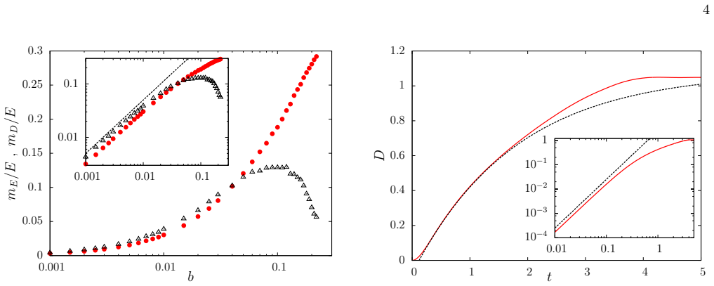
The ratio of maximum error growth rate to maximum separation growth rate $m_E/m_D$ is near $1.35$ at low $b$, consistent with the error being bounded by $2D$.
Homogeneous isotropic turbulence at $\mathrm{Re} = 490$ shows the same $D(t)$ curve, suggesting that the constrained-random-walk description extends to hydrodynamic turbulence.
The qualitatively different error-growth regimes seen in turbulence—linear growth in three dimensions with dissipation, and random-walk-like behavior in two dimensions with low dissipation—mirror the two regimes found in the cyclically symmetric attractor, hinting at a universal energy-constrained behavior.

Reading between the lines

Editorial extensions of the paper, not claims the author makes directly.

If the random-walk description is exact, the effective diffusion time $\tau$ should be derivable from the attractor's Lyapunov spectrum and energy fluctuations; the paper does not derive it, so a parameter-free prediction of $\tau$ would be a direct test.
The same $D = 2E(1 - \exp(-t/\tau))$ form should appear in other bounded high-dimensional chaotic systems, such as shell models of turbulence or the Kuramoto–Sivashinsky equation, whenever the energy is approximately conserved.
The bound $E_d \leq 2D$ implies a practical ceiling on ensemble forecasting in high-dimensional systems: once the separation saturates, two forecasts are no further apart than the system's own wandering, which could set a floor on useful prediction horizons.
Observational data (for example, atmospheric reanalyses) could be searched for this signature by testing whether the mean squared difference between two analyses follows the exponential-saturation curve rather than unbounded growth.

Share X Bluesky LinkedIn Reddit HN

Signed reviews

No signed human review yet.

Editorial analysis

A structured set of objections, weighed in public.

Desk editor's note, referee report, and a circularity audit.

Desk Editor's Note

read the letter

Hi [Name],

Quick take on 1908.05989: the headline claim—that high-dimensional TCSA and homogeneous isotropic turbulence behave like a random walk constrained on a hypersphere—is plausible, but the evidence as presented is a fit, not a parameter-free test. The random-walk-on-sphere section itself is clean and correct; the soft spots are all in Sections III and IV.

What's new: extending the Thomas cyclically symmetric attractor to b>0 and showing that D(t) saturates like 2E(1-exp(-t/tau)) while the error Ed(t) switches from linear growth at moderate b to D-bounded growth at low b. The b=0 case already had random-walk behavior from Sprott and Chlouverakis; the b>0 observation and the qualitative turbulence link are the genuine additions.

The strength is the random walk section. They simulate a constrained random walk in 100,000 dimensions, measure D, and recover 1/tau = s/2. That part works.

The soft spots: in Section III, tau for TCSA is never derived from Eq. (6). The dashed curve in Fig. 2 is drawn with an 'effective' tau and 'a slight offset of time.' No fitting procedure, no error bars, no independent prediction. A saturating exponential with two free parameters can match any bounded ergodic observable with roughly exponential correlation decay, so the match doesn't distinguish a constrained random walk from generic bounded-chaos dynamics. Same issue in Fig. 6 for turbulence: the dashed line is 'a comparison to Eq. (2)' but how tau was obtained isn't stated. The low-b error bound is also heuristic: the text says Ed is bounded by 2D, but by the triangle inequality the squared-error bound is Ed <= 4D. The qualitative argument survives, but the stated constant is off.

Is the central argument salvageable? Yes, the qualitative behavior is there. But the paper needs to either derive tau from the equations of motion or explicitly present it as an empirical fit, and then discuss what that fit does and doesn't buy. They also need to correct the 2D vs 4D point and give error bars on mE/mD.

This is a paper for people working on chaos and turbulence predictability. It deserves a serious referee, but with the expectation of major revision. The referee should press on the tau fitting and the bound.

My recommendation: engage with it as a conditional. Send it to review; it's not a desk reject. But it needs work before the central claim is convincing.

— [Your name]

Referee Report

3 major / 5 minor

Summary. The manuscript studies the hypothesis that high-dimensional chaotic systems with an approximate energy constraint behave like random walks constrained to a hypersphere in state space. Section II derives and numerically verifies that the squared displacement D(t) of a random walk on the surface of an n-dimensional unit sphere follows D(t)=2E(1-exp(-t/tau)), with the diffusion time determined by the step statistics. Section III applies this idea to an n-dimensional Thomas cyclically symmetric attractor (TCSA), claiming that for b=0.1 the field difference D(t) follows Eq. (2) after a small time offset and that the error Ed(t) grows linearly, while for b=0.001 the error itself is limited by the random-walk behavior. Section IV compares D(t) from a direct numerical simulation of homogeneous isotropic turbulence at Re=490 with Eq. (2) and reports qualitative agreement, suggesting a universal predictability limit for energy-bounded chaotic systems.

Significance. The central idea is attractive and potentially useful: if the late-time behavior of D(t) and error growth in high-dimensional chaotic systems is governed by diffusion on a constant-energy hypersphere, predictability limits could be understood from a simple geometric picture. The random-walk-on-a-hypersphere section is a clean, essentially parameter-free test of Eq. (2), since tau is set by the prescribed step statistics, and Fig. 1 shows good agreement. The qualitative distinction between linear error growth at moderate damping and random-walk-limited error at low damping in TCSA is interesting and connects to known turbulence results. However, the application sections currently establish only that D(t) and Ed(t) resemble saturating exponentials with a fitted tau and a time offset; without a prediction of tau from the system parameters, the empirical match is a fit rather than a test, which limits the strength of the claimed universality.

major comments (3)

[§III, Fig. 2 and Fig. 4] The comparison of the TCSA D(t) to Eq. (2) uses an 'effective' diffusion time tau and a 'small offset of time', but neither the values of tau and the offset nor the fitting procedure are given, and tau is not derived from Eq. (6). Because Eq. (2) is a saturating exponential, a two-parameter fit with tau and an offset can describe many bounded signals with finite correlation time; as presented, the agreement does not discriminate between a constrained random walk and generic bounded chaotic dynamics. Please derive tau from the TCSA equations (for example, from the autocorrelation of sin(x_i) or from the linearized dynamics) and compare its predicted value with the simulation, or at minimum report the fitted tau and show that it varies with b in a meaningful way.
[§IV, Fig. 6] The turbulence D(t) is compared with Eq. (2) using a dashed line, but the text does not state how tau was obtained, what the fit range was, or what uncertainty the comparison carries. The same fitting concern as in §III applies, and it is especially important here because the turbulence data are taken from another study [9] and the reader cannot judge whether the agreement is a post hoc fit. Please specify the tau used, and ideally connect it to known turbulence time scales such as the integral or eddy-turnover time.
[§III, near Eq. (7) and Fig. 5] The heuristic bound states that 'the bound on Ed is 2D'. Since D(t) and Ed(t) are defined as squared distances (Eqs. (4) and (7)), the triangle inequality gives sqrt(Ed(t)) <= sqrt(D(t)) + sqrt(D(t)), hence Ed(t) <= 4D(t), not 2D(t). The factor error should be corrected; the qualitative conclusion that Ed is bounded by a constant multiple of D is unchanged, but the stated numerical factor 2 is wrong.

minor comments (5)

[§II, after Eq. (3)] The statement that the Euclidean norm of the step vector has |r| = s is incorrect; a vector with n components each of magnitude sqrt(s/n) has norm sqrt(s). The convention s = |r|^2 is consistent with the reported 1/tau = s/2 and with Eq. (2), but the text should call s the squared step length and correct this identity.
[Eq. (1)] The use of 'cos(theta) ~ exp(-t/tau)' should specify the sense of the approximation (for example, ensemble average for large n and small step) and whether tau is in time units or in steps.
[§III, Fig. 5] The 'maximum gradient' mE and mD is not defined; please specify how the maximum slope is extracted from the noisy curves (for example, smoothing or windowing), so that the reported ratios such as mE/mD = 1.35 +/- 0.04 are reproducible.
[§IV] The manuscript states Re = 490 but does not describe the grid resolution or numerical method; since the data are borrowed from [9], a brief description of the simulation parameters would help the reader assess the comparison.
[References] Reference [11] has a typo in the author name ('Musachhio' should be 'Musacchio').

Circularity Check

2 steps flagged · score 6.0 of 10

The TCSA and turbulence supports for Eq. (2) are fits: the diffusion time τ and a time offset are chosen to make the dashed curve match D(t), so the central 'random walk' agreement is partly by construction.

fitted input called prediction [Section III, Fig. 2 caption and text following Eq. (6)]
"However, for high t, D behaves similar to the prediction for a random walk on a hypersphere given in Eqn. (2), but with a slight offset of time. ... Dashed black line is the expected behaviour of a random walk on a sphere, offset by a small time."

The dashed 'expected' curve is Eq. (2) evaluated with an unspecified τ and an unspecified time offset. No derivation of τ from the TCSA equations (6) or from b is given anywhere in the paper; the only way to draw the dashed curve is to choose τ and the offset to match the simulated D(t). The agreement is therefore constructed by fitting the very quantity it is used to predict. A saturating exponential with a free rate and a free time shift can be matched to almost any bounded, initially increasing observable, so this comparison does not independently test the random-walk-on-hypersphere mechanism.
fitted input called prediction [Section IV, Fig. 6 caption and text]
"As can be seen from the figure, the growth of D is well approximated as following the prediction in Eqn. (2). ... Red (grey) solid line is measured D and dashed black line is a comparison to Eqn. (2)."

The turbulence comparison uses Eq. (2) as the dashed line but does not state how τ (or E) was obtained for the Re=490 simulation. No derivation of τ from the Navier-Stokes parameters is provided. The dashed curve is thus a fitted version of Eq. (2), and the agreement with the measured D is not an independent prediction. The admitted late-time departure due to non-constant energy further shows that the comparison relies on adjustable normalization.

full rationale

The random-walk-on-hypersphere section itself is non-circular: the step rule (3) and the stated 1/τ=s/2 relation define the model, and Fig. 1 tests Eq. (2) against a simulation of that model. The circularity enters when the same Eq. (2) is used as the 'expected behaviour' for TCSA and turbulence: τ and a time offset are never derived from the dynamics, so the dashed lines in Figs. 2, 4, and 6 are fits to the D(t) curve they are supposed to validate. This matches the fitted-input-called-prediction pattern and makes the central random-walk claim for the chaotic systems partially circular. The self-citations (e.g., [9]) are not load-bearing in a circular way: they supply simulation data and earlier linear-error results, but do not themselves assert the constrained-random-walk interpretation. Also, the heuristic bound Ed≤2D in Section III is dimensionally suspect (for squared distances the triangle inequality gives Ed≤4D), but that is a correctness issue rather than circularity. Overall score 6 because one or more central 'predictions' reduce by construction, while the random-walk model itself retains independent content.

Assumptions & free parameters 3 free parameters · 4 assumptions · 0 invented entities

The central comparisons rest on an effective time scale τ that is not derived for TCSA or turbulence, plus a heuristic bounding argument for the error. The random walk on a sphere formula itself is standard.

free parameters (3)

Effective diffusion time τ for TCSA = not stated
In Fig. 2, D(t) for the TCSA is compared to Eq. (2) with a 'slight offset of time'; τ is not derived from the system parameters (b, n, etc.) and is effectively fitted to the simulated D(t).
Effective diffusion time τ for turbulence = not stated
In Fig. 6, D(t) from the turbulence simulation is compared to Eq. (2); τ is not derived from Re or any flow quantity and is an effective fit.
Time offset for TCSA comparison = not stated
The dashed line in Fig. 2 is described as 'offset by a small time'; this offset is an additional adjustable quantity in the comparison.

assumptions (4)

standard math A random walk on a unit hypersphere has cos(θ) ~ exp(-t/τ) (Eq. 1).
Taken from Caillol [3]; used as the basis for Eq. (2) and the comparisons in Figs. 1, 2, and 6.
domain assumption For b > 0, the energy E of the TCSA varies only slightly, so the dynamics can be treated as a random walk on a constant-energy hypersphere.
State in Section III: 'for b > 0, E varies only slightly.' This justifies applying Eq. (2) to the TCSA.
domain assumption The b=0 TCSA behaves like a random walk with independent and identically distributed steps.
Based on prior work [5,6]; used to motivate the analogy for b>0.
ad hoc to paper The error Ed(t) is bounded by 2D(t) (or proportional to D(t)) because two nearby states can be at most twice the distance from a reference state.
Heuristic argument in Section III after Fig. 4; used to explain why Ed follows D for low b. Not rigorously derived.

how reviews work

0 comments

Cite this review

Pith. "Pith review of High dimensional chaotic systems which behave like random walks in state space." pith.science (2026). https://pith.science/paper/H5LPAXPT

@misc{pith2026190805989,
  author       = {Pith},
  title        = {Pith review of: High dimensional chaotic systems which behave like random walks in state space},
  year         = {2026},
  howpublished = {\url{https://pith.science/paper/H5LPAXPT}},
  note         = {Machine review of arXiv:1908.05989}
}

read the original abstract

By analysing an n-dimensional generalisation of Thomas's cyclically symmetric attractor we find that this chaotic dynamical system behaves like a random walk constrained onto the surface of a hypersphere. The growth of error is limited, with qualitatively different behaviour depending on a control parameter. For moderate values of the control parameter, linear growth of error is seen. For low values of the control parameter, the error is limited by the random walk behaviour. Finally, we link this to the predictability of homogeneous isotropic turbulence, which we find here also behaves like a constrained random walk.

Figures

Figures reproduced from arXiv: 1908.05989 by the authors.

**Figure 2.** FIG. 2: Difference, [PITH_FULL_IMAGE:figures/full_fig_p003_2.png] view at source ↗

**Figure 3.** FIG. 3: Error, [PITH_FULL_IMAGE:figures/full_fig_p003_3.png] view at source ↗

Figures from the paper (1 more)

**Figure 5.** Figure 5: FIG. 5: Maximum gradients [PITH_FULL_IMAGE:figures/full_fig_p004_5.png]

Discussion (0). Continue with ORCID to comment.

Reference graph

Works this paper leans on

13 extracted references · 12 canonical work pages

[9]

Berera and R

A. Berera and R. D. J. G. Ho, Phys. Rev. Lett. 120, 024101 (2018)

2018
[1]

E. N. Lorenz, J. Atmos. Sci. 20, 130 (1963)

work page 1963
[2]

E. N. Lorenz, Tellus 21, 289 (1969)

work page 1969
[3]

Caillol, J

J-M. Caillol, J. Phys. A: Math. Gen. 37, 3077 (2004)

work page 2004
[4]

Thomas, Int

R. Thomas, Int. J. Bifurc. Chaos 9, 1889 (1999)

work page 1999
[5]

J. C. Sprott, K. E. Chlouverakis, Int. J. Bifurc. Chaos 17, 2097 (2007)

work page 2007
[6]

K. E. Chlouverakis, J. C. Sprott, Chaos 17 023110 (2007)

work page 2007
[7]

Eckhardt, T

B. Eckhardt, T. M. Schneider, B. Hof, and J. Westerweel, Annu. Rev. Fluid Mech. 39, 447 (2007)

work page 2007

Show all 13 references

[8]

Lemoult, L

G. Lemoult, L. Shi, K. Avila, S. V. Jalikop, M. Avila, and B. Hof, Nature Phys. 12, 254 (2016)

2016
[10]

Boﬀetta and S

G. Boﬀetta and S. Musacchio, Phys. Rev. Lett. 119, 054102 (2017)

2017
[11]

Boﬀetta and S

G. Boﬀetta and S. Musachhio, Phys. Fluids 13, 1060 (2001)

2001
[12]

ARCHER, http://www.archer.ac.uk
[490]

As can be seen from the ﬁgure, the growth of D is well approximated as following the prediction in Eqn

The details of this simulation are the same as those used for the main results in [9]. As can be seen from the ﬁgure, the growth of D is well approximated as following the prediction in Eqn. (2). The departure from predic- tion at later time is due to the fact that the assumpt...

Pith tools

Reviewed August 14, 2026 · model on record in the stance chip above.

[1] [9]

Berera and R

A. Berera and R. D. J. G. Ho, Phys. Rev. Lett. 120, 024101 (2018)

2018

[2] [1]

E. N. Lorenz, J. Atmos. Sci. 20, 130 (1963)

work page 1963

[3] [2]

E. N. Lorenz, Tellus 21, 289 (1969)

work page 1969

[4] [3]

Caillol, J

J-M. Caillol, J. Phys. A: Math. Gen. 37, 3077 (2004)

work page 2004

[5] [4]

Thomas, Int

R. Thomas, Int. J. Bifurc. Chaos 9, 1889 (1999)

work page 1999

[6] [5]

J. C. Sprott, K. E. Chlouverakis, Int. J. Bifurc. Chaos 17, 2097 (2007)

work page 2007

[7] [6]

K. E. Chlouverakis, J. C. Sprott, Chaos 17 023110 (2007)

work page 2007

[8] [7]

Eckhardt, T

B. Eckhardt, T. M. Schneider, B. Hof, and J. Westerweel, Annu. Rev. Fluid Mech. 39, 447 (2007)

work page 2007