Arrow diagrams on spherical curves and computations

Masashi Takamura; Noboru Ito

REVIEW 3 major objections 4 minor 16 references

Arrow diagrams on spherical curves and computations

T0 review · 3 major / 4 minor · reviewed 2026-08-14 · deepseek-v4-flash

Challenge this review Re-run · record.json Download PDF Read on arXiv ↗ Review JSON

Pith's one-line read The paper proves that arrow-diagram counting functions become spherical-curve invariants when a delta-version vanishes on relators, and computes such invariants through six arrows.

desk verdict New relator framework for spherical-curve invariants; computational section is promising but needs a clearer match between the solved linear system and Theorem 1. read the letter →

arxiv 1908.06085 v1 pith:Z6GZ7YUE submitted 2019-08-16 math.GT

Noboru Ito , Masashi Takamura This is my paper · ORCID

classification math.GT MSC 57M2757M25

keywords sphericalcurvesarrowdiagramsorientedGausswordsReidemeistermovesweak(13)homotopyfinitetypeinvariantsnormal

verification ladder T0 review T1 audit T2 compute T3 formal

The pith

A machine-rendered reading of the paper's core claim, the machinery that carries it, and where it could break.

The reading

Spherical curves are generic circle immersions into the 2-sphere, studied up to five Reidemeister-style deformations: RI, strong and weak RII, and strong and weak RIII. The paper establishes a general criterion for turning arrow-diagram counting functions into integer-valued invariants under any chosen combination of those moves: one checks a much simpler delta-function version against a finite list of formal relators, and the check guarantees invariance. The authors then compute by enumerating normal oriented Gauss words and taking kernels of the resulting relator matrices. For weak (1,3) homotopy—RI together with weak RIII—the computation yields dimensions 1, 3, 13, 31 at successive arrow counts, including the explicit three-arrow invariant $-x^*_1+x^*_2-x^*_3-x^*_4-x^*_5-x^*_6+3x^*_7$. The motivation is an open question about whether the map taking a spherical curve to its positive knot diagram is injective under this homotopy.

What carries the argument

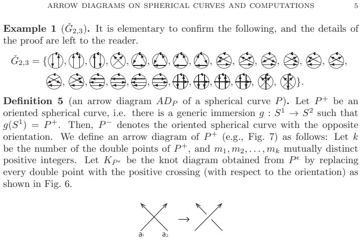
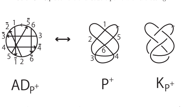
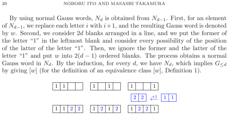
The key object is the arrow diagram, here identified with an oriented Gauss word: a cyclic word in which each letter occurs twice, once marked as a starting point and once as an end point. For each isomorphism class $x^*_i$, the function $x^*_i(AD)$ counts how many sub-arrow-diagrams of $AD$ are isomorphic to $x^*_i$, while $\tilde{x}^*_i$ is the Kronecker delta on that single isomorphism class. The identity $x^*_i(AD)=\sum_{z^*\in\mathrm{Sub}(G^*)}\tilde{x}^*_i(z^*)$ reduces every Reidemeister-style deformation to a difference of such sums, and the relators are exactly those differences written as elements of the free $\mathbb{Z}$-module on arrow diagrams. The computational engine is the enumeration of normal oriented Gauss words—words whose first occurrences of letters read $1,2,\dots,n$ in order—by inserting the first letter into all possible positions and then lexicographically assigning orientations; the kernel of the resulting matrix $(\tilde{x}^*_i(r^*_j))$ is the space of invariants.

What would settle it

Run an independent enumeration of connected normal oriented Gauss words with five and six arrows and recompute the rank of the weak-RIII relator matrix; if the number of isomorphism classes in $\check{G}_{5,6}\cap\mathrm{Conn}$ is not 15,922 or the kernel dimension is not 31, the paper's computational claim fails. For the three-arrow stage the matrix is printed in full, so the kernel can also be checked by hand.

Watch

Extended reading notes

Core claim

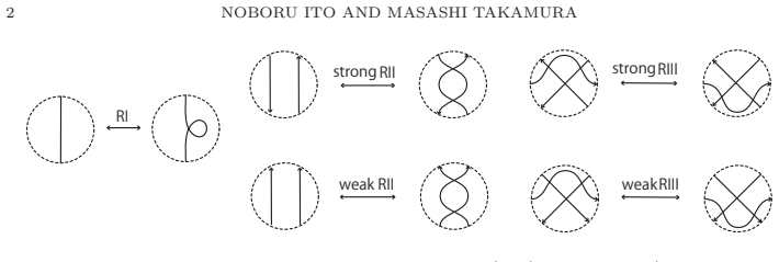
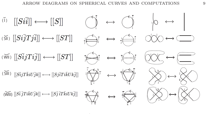
The central result (Theorem 1) is a transfer principle. Fix two arrow-count bounds $b,d$ and a subset of the five move types, encoded by $(\epsilon_1,\dots,\epsilon_5)\in\{0,1\}^5$, and form the finite set of relators $\check{R}_{\epsilon}(b,d)$ obtained by projecting the Type ($\check{\mathrm{I}}$), strong/weak ($\check{\mathrm{II}}$), and strong/weak ($\check{\mathrm{III}}$) relators to arrow diagrams with between $b$ and $d$ arrows. If a linear combination $\sum\alpha_i\tilde{x}^*_i$ of delta functions on arrow-diagram isomorphism classes vanishes on every relator in the selected family, then the corresponding counting function $\sum\alpha_i x^*_i$ is an integer-valued invariant of oriented spherical curves under the corresponding deformations; a mirroring-pair condition makes the invariant independent of orientation. Computers then compute the kernel dimensions of the matrices $(\tilde{x}^*_i(r^*_j))$. For weak (1,3) homotopy the dimensions are $\dim V^{\mathrm{ori}}_w(2,3)=1$, $\dim V^{\mathrm{ori}}_w(3,4)=3$, $\dim V^{\mathrm{ori}}_w(4,5)=13$, and $\dim V^{\mathrm{ori}}_w(5,6)=31$; the paper also lists the explicit coefficients $-x^*_1+x^*_2-x^*_3-x^*_4-x^*_5-x^*_6+3x^*_7$ at the three-arrow stage and notes, citing the finite-type invariant literature, that this particular one vanishes on spherical curves. For RI together with strong RIII the computed dimensions are 3, 18, 145.

Load-bearing premise

The computed dimensions and coefficient tuples rest on the completeness and duplicate-freeness of the enumeration of normal oriented Gauss words in Section 4; the paper spells out the procedure but gives no formal proof or independent audit of the enumeration, and the raw lists for the five- and six-arrow cases are not printed in the paper.

Editorial extensions

If this is right

Any kernel vector of a relator matrix yields an integer-valued invariant, so the paper converts the search for invariants under any of the 32 equivalence relations generated by the five moves into a finite linear-algebra computation.
The weak (1,3) homotopy dimensions 1, 3, 13, 31 show new invariants appear at each successive arrow-count stage through six arrows; the paper conjectures these dimensions never exceed the corresponding knot-theoretic finite-type invariant dimensions.
Restricting to connected arrow diagrams (Corollary 2) makes the invariants additive under connected sum, so the computed invariants behave like finite-type invariants with respect to connect-sum decomposition.
The explicit three-arrow invariant, even though it vanishes on spherical curves according to the cited review, gives a pattern that the 13- and 31-dimensional spaces refine, and it provides a concrete check for any independent implementation.

Reading between the lines

Editorial extensions of the paper, not claims the author makes directly.

The same relator-kernel computation can be run for any other subset of the five move types, including mixed combinations such as RI plus strong RII plus weak RIII, so the method is a general source of invariants for all 32 equivalence relations once the normal oriented Gauss word enumeration is available.
A direct next step is to evaluate the 13- and 31-dimensional invariants on the prime spherical curves with up to seven double points; if they take equal values on curves like 7_4 and 7_B, the filtration remains coarse at this order, while any separation would give the first computational evidence about the injectivity question that motivates the paper.
Because the relator matrices depend only on the inclusion poset of arrow diagrams, the same enumeration and matrix data can be reused when the move set changes, so the computational cost is amortized across many equivalence relations at once.

Share X Bluesky LinkedIn Reddit HN

Signed reviews

No signed human review yet.

Editorial analysis

A structured set of objections, weighed in public.

Desk editor's note, referee report, and a circularity audit.

Desk Editor's Note

read the letter

Dear colleague,

Two things to know about arXiv:1908.06085. First, the relator framework is a genuinely useful way to generate invariants of spherical curves under any of the 32 equivalence relations from the five move types. Theorem 1 is a clean sufficient condition: vanish on the relators with the tilde functions and you get an invariant. The proof for RI, strong RII, and strong RIII is direct and looks correct; the weak RII and weak RIII cases are omitted as “essentially the same,” which is a minor but real gap.

Second, the computational section is not as cleanly tied to Theorem 1 as it should be. The stress-test note that reached me claims Example 9 solves a different system because the matrix A uses x*_i (subword counts) instead of x̃*_i. I checked the example: that particular claim is wrong. In R00010(2,3) the relators are projected to diagrams with at most three arrows, and the x_i are the connected three-arrow diagrams, so for these terms x_i(r) is just the coefficient of x_i in r—same as x̃*_i(r). The entry 3 in the first row is a multiplicity, not a subword count, and the relator does not have empty S,T,U as the note says.

But the general issue survives. For b≥3, ČG_{b,b+1} includes diagrams of two different sizes, and a relator term with b+1 arrows can contain several sub-diagrams of size b. Then x_i(r) genuinely differs from the coefficient of x_i in r, and the kernel of the matrix is not obviously the same as the kernel of the tilde evaluation used in Theorem 1. The paper doesn’t address this. It may be that the code actually computes coefficients and the dimension table is fine, but the written definition of the matrix and the appeal to Corollary 2 need explicit justification.

The other soft spots are minor: the enumeration in Section 4 needs a proof of completeness, and the data for n=5,6 lives on an external webpage with no shipped code. For a theorem-driven computation paper, that’s a reproducibility issue, not a fatal one.

Who it’s for: people working on knot projections or finite-type invariants from Gauss diagrams. It deserves a serious referee. I’d send it out and ask for the missing proofs, a clarified matrix definition, and archived code/data.

Best,

Referee Report

3 major / 4 minor

Summary. The paper introduces integer-valued functions on oriented spherical curves of the form Σ α_i x*_i, where x*_i(AD) counts the number of sub-arrow-diagrams of AD isomorphic to a fixed arrow diagram x*_i. It also defines auxiliary functions Σ α_i x̃*_i that read off coefficients in the free Z-module generated by arrow diagrams, and it defines five families of relators corresponding to the deformations RI, strong RII, weak RII, strong RIII, and weak RIII. Theorem 1 states that if Σ α_i x̃*_i vanishes on all projected relators of the selected deformation types, then Σ α_i x*_i is an invariant under those deformations. The proof is carried out explicitly for RI, strong RII, and strong RIII; the weak RII and weak RIII cases are omitted as "essentially the same." The computational part of the paper enumerates normal oriented Gauss words, reports kernel dimensions of a matrix A=(x*_i(r*_j)), and in particular claims dim V_ori_w(5,6)=31 and an explicit weak (1,3) homotopy invariant; the raw data for n=5,6 is posted on an external webpage.

Significance. If the results stand, the paper provides a clean and systematic machine-assisted source of sub-arrow-diagram count invariants for spherical curves, including invariants under weak (1,3) homotopy, and it gives concrete computational evidence relevant to the Kamada–Nakanishi Question 1. The theoretical criterion in Theorem 1 is attractive, and the written proofs for the RI, strong RII, and strong RIII cases are direct combinatorial cancellations that are easy to follow. The paper also deserves credit for printing explicit matrices, relators, and invariants for small arrow numbers rather than leaving everything to opaque code. However, the central computational claim currently rests on a linear system that does not match the hypothesis of Theorem 1, and it is not accompanied by audited code or by complete data for the largest computation, so the reported dimensions and invariants are not yet established.

major comments (3)

[Section 4.2, Examples 9–10] The matrix A is defined as A=(x*_i(r*_sj)), and the reported invariants are obtained from α^T A=0. But Theorem 1 requires Σ α_i x̃*_i(r*)=0 for every relator r*, where x̃*_i(r*) is the coefficient of the diagram x*_i in the linear combination r*. The quantity x*_i(r*) is different: it is the signed sum, over all terms of r*, of the number of sub-diagrams of each term isomorphic to x*_i. These two functionals are not equal. For example, in the strong-RIII relator of Definition 7 with S=T=U=∅, the 2-arrow diagram [[¯ij i¯j]] has coefficient +1 in the relator, but it also occurs as a sub-diagram of the 3-arrow term [[¯ij¯ki¯jk]], so x*([[¯ij i¯j]])(r)=2 while x̃*([[¯ij i¯j]])(r)=1. Thus the matrix solved in Examples 9 and 10 is not the coefficient matrix required by Theorem 1 unless an additional transformation is supplied, and no such transformation is mentioned. The reported dimensions, including dim V_ori_w(5,6)=31, and the displayed weak (1,3) homotopy invariant are therefore not justified as stated by the paper's own theorem.
[Section 3, cases ǫ3=1 and ǫ5=1] The proofs for weak RII and weak RIII are omitted with the remark that the arguments are essentially the same as the strong cases. Since weak RII and weak RIII are part of the statement of Theorem 1 and are central to the paper's stated goal of obtaining weak (1,3) homotopy invariants, this is a gap in the proof of a load-bearing result. The authors should either include the omitted arguments or state and prove a precise reduction showing that the weak cases follow word-for-word from the strong cases.
[Section 4.1–4.2 and Section 5] The completeness and duplicate-freeness of the enumeration of normal oriented Gauss words in Steps 1–5 is asserted without proof or machine-checkable certificate. The claims dim V_ori_w(4,5)=13 and dim V_ori_w(5,6)=31 depend entirely on this enumeration being exact, and the raw list for n=5,6 is only available at an external webpage rather than in the paper or in an audited program. Even after the matrix question in Examples 9–10 is resolved, the computational results need a reproducibility mechanism, such as the source code, the raw enumeration, or a certificate that can be checked independently.

minor comments (4)

[Abstract and Theorem 1] The abstract says that vanishing of Σ α_i x̃*_i implies Σ α_i x̃* is invariant, but the invariant is Σ α_i x*_i; this is presumably a typo and should be corrected.
[Definition 1] The definition of a sub-word appears to define only suffixes of prefixes of w, namely u(j)=w(n-p+j), whereas Definition 3 and the rest of the paper use sub-words obtained by deleting pairs of letters. Please correct the formal definition to match the intended deletion operation.
[Section 4.1] The text says the computation uses C++11 and Mathematica, but no code, version numbers, or numerical linear algebra details are provided; adding this information would substantially improve reproducibility.
[Tables 7–19] The thirteen invariant tuples in Tables 7–19 are printed without a clear statement of which column index corresponds to which diagram in Tables 4–6; a short example explaining how to read the tuples would make the tables usable.

Circularity Check

0 steps flagged · score 0.0 of 10

No significant circularity: the invariants are derived from an independent indicator function and the relators are defined from Reidemeister moves, not from the invariants.

full rationale

The paper's derivation is self-contained and does not exhibit circularity. Theorem 1 starts from the independently defined indicator function $\tilde{x}^*_i$ (Definition 6) and shows that vanishing of $\sum\alpha_i\tilde{x}^*_i$ on relators (Definition 7, which are formal combinations dictated by Reidemeister moves) forces invariance of the subword-count combination $\sum\alpha_i x^*_i$ via equation (1), $x^*_i(AD)=\sum_{z^*\in\mathrm{Sub}(G^*)}\tilde{x}^*_i(z^*)$; the relators are not defined in terms of the invariants, and the coefficients $\alpha$ are solutions of a linear system rather than fitted parameters. The self-citations (e.g., [7], [9], [11], [13]) are contextual or used for auxiliary moves and tables; none is load-bearing for the main theorem. One separate, non-circular concern is that Examples 9-11 set $A=(x^*_i(r^*_{sj}))$ and solve $xA=0$, whereas Theorem 1's hypothesis is stated with $\tilde{x}^*_i$; these coincide in the displayed $b=2,d=3$ setting because all basis diagrams have exactly three arrows and no relator term has more than three arrows, but for the $(5,6)$ table this equivalence is not shown. That is a correctness or verification gap, not a self-referential reduction.

Assumptions & free parameters 0 free parameters · 3 assumptions · 0 invented entities

The paper's central construction depends on standard Reidemeister-type equivalence for spherical curves, the correspondence between oriented Gauss words and arrow diagrams, and the assertion that the relators faithfully encode the five local moves. These are background facts from the literature, not derived in the paper. No free parameters are fitted; the α_i are variables in a homogeneous linear system, and the authors solve for the kernel.

assumptions (3)

domain assumption Equivalence classes of (oriented) Gauss words of length 2n are in one-to-one correspondence with (arrow) chord diagrams.
Stated in Section 2.1 after Definitions 4 and 5; used throughout to identify arrow diagrams with oriented Gauss words.
domain assumption Any two spherical curves are related by a finite sequence of RI, RII, and RIII deformations.
Invoked in the introduction and in Theorem 1 to reduce ambient isotopy to local moves; cited from the literature [1], [11].
domain assumption The relators of Types I, SII, WII, SIII, and WIII correspond exactly to single deformations RI, strong RII, weak RII, strong RIII, and weak RIII.
Stated after Definition 7; the correspondence is asserted and used to convert vanishing on relators into invariance under the moves.

how reviews work

0 comments

Cite this review

Pith. "Pith review of Arrow diagrams on spherical curves and computations." pith.science (2026). https://pith.science/paper/Z6GZ7YUE

@misc{pith2026190806085,
  author       = {Pith},
  title        = {Pith review of: Arrow diagrams on spherical curves and computations},
  year         = {2026},
  howpublished = {\url{https://pith.science/paper/Z6GZ7YUE}},
  note         = {Machine review of arXiv:1908.06085}
}

abstract

We give a definition of an integer-valued function $\sum_i \alpha_i x ^*_i$ derived from arrow diagrams for the ambient isotopy classes of oriented spherical curves. Then, we introduce certain elements of the free $\mathbb{Z}$-module generated by the arrow diagrams with at most $l $ arrows, called relators of Type~($\check{\rm{I}}$) (($\check{\rm{SI\!I} }$), ($\check{\rm{WI\!I}}$), ($\check{\rm{SI\!I\!I}}$), or ($\check{\rm{ WI\!I\!I}}$), resp.), and introduce another function $\sum_i \alpha_i \tilde{x}^*_i$ to obtain $\sum_i \alpha_i x^*_i$. One of the main results shows that if $\sum_i \alpha_i \tilde{x}^*_i$ vanishes on finitely many relators of Type~($\check{\rm{I}}$) (($\check{\rm{SI\!I}}$) , ($\check{\rm{WI\!I}}$), ($\check{\rm{SI\!I\!I}}$), or ($\check{\rm{WI\! I\!I}}$), resp.), then $\sum_i \alpha_i \tilde{x}$ is invariant under the deformation of type $\rm{RI}$ (strong$\rm{RI\!I}$, weak$\rm{RI\!I}$, strong$\rm{RI\!I\!I}$, or weak$\rm{RI\!I\!I}$, resp.). The other main result is that we obtain functions of arrow diagrams with up to six arrows. This computation is done with the aid of computers.

Figures

Figures reproduced from arXiv: 1908.06085 by the authors.

**Figure 1.** Deformations of three types: RI, RII, and RIII. moves of type Ω1, Ω2, and Ω3 on knot diagrams by ignoring over/under information of double points. It is known that a finite number of repetitions of Reidemeister moves suffice to take any one diagram of a knot to any other. Deformations of 5 types arise 32 (= 25 ) equivalence relations. By [11], it is known that 32 equivalence relations arise a non-trivial classificat… view at source ↗

**Figure 2.** Deformations of five types: RI (left), strong RII (upper center), weak RII (lower center), strong RIII (upper right), weak RIII (lower right) [PITH_FULL_IMAGE:figures/full_fig_p002_2.png] view at source ↗

**Figure 3.** The replacement of a double point to the positive crossing Here, every crossing of the type as in the rightmost figure of [PITH_FULL_IMAGE:figures/full_fig_p002_3.png] view at source ↗

Figures from the paper (13 more)

**Figure 4.** Figure 4: Four expressions (Gauss words and chord diagrams). We note that the equivalence classes of the Gauss words of length 2n have one to one correspondence with a chord diagrams, each of which has n chords. We identify these four expressions ( [PITH_FULL_IMAGE:figures/full…

**Figure 5.** Figure 5: Four expressions (oriented Gauss words and arrow diagrams). Here, we note that, in general, v ∗ and v ∗ ◦ rev are not isomorphic, and this implies that an arrow diagram and its reflection image are not ambient isotopic in general. Thus, in this paper, we express this c…

**Figure 6.** Figure 6: Replacement of a double point with a crossing. P KP + + ADP + 1 2 3 4 5 6 1 1 2 2 3 3 4 4 5 5 6 6 [PITH_FULL_IMAGE:figures/full_fig_p005_6.png]

**Figure 7.** Figure 7: An arrow diagram ADP of an oriented spherical curve P +. Fix a base point, which is not a double point on KP + . Starting from the base point, proceed along P + according to the orientation of KP + . Assign m1 to the first double point that we encounter. Then, assign m…

**Figure 8.** Figure 8: ( AD ) ( AD ) ( AD ) ( AD ) ( AD ) ( AD ) ( AD ) = = = 3 = 4 11 = 4 4 = 1 = 1 AD = α α α α α α 1 2 3 4 5 6 [PITH_FULL_IMAGE:figures/full_fig_p006_8.png]

**Figure 9.** Figure 9: x ∗ (P +). By definition, it is easy to see x˜∗(F ∗ 1 ) = x˜∗(F ∗ 2 ) for each pair F ∗ 1 , F ∗ 2 with [[F ∗ 1 ]] = [[F ∗ 2 ]]. Hence, we shall denote this number by x˜∗([[F ∗ 1 ]]). If [[F ∗ ]] corresponds to an arrow diagram of an oriented spherical curve P ǫ , then …

**Figure 10.** Figure 10: Relators. We note that in Definition 7, if the oriented Gauss word G∗ is obtained from an oriented spherical curve P ǫ , then each relator corresponds to a deformation: Type ( ˇI) relator to RI, Type (SII) relator to strong RII, Type ( ˇ WII) relator to weak RII, ˇ Ty…

**Figure 11.** Figure 11: Deformations (the mirror images of the center and the corresponding words are omitted). arises from i, j, and k. Then, (3) Subx∗ (G ∗ ) = Sub(0) x∗ (G ∗ ) ∐ Sub(1) x∗ (G ∗ ) ∐ Sub(2) x∗ (G ∗ ) ∐ Sub(3) x∗ (G ∗ ). Let Cˇ be the set of the ambient isotopy classes of ori…

**Figure 12.** Figure 12: N2 is obtained by N1. Next, we enumerate elements in Rˇ 00001. Let us start with a toy model of a linear sum of unoriented Gauss words. Let S, T , and U be sub-words where ST U is a Gauss word. Then, let r = ([Si jT ikU jk] + [Si jT iU j] + [SiT ikU k] + [SjT kU jk]) …

**Figure 13.** Figure 13: The chord diagram corresponding to 12Si1T i2U (i = 3). add a single letter (corresponding to a chord as in [PITH_FULL_IMAGE:figures/full_fig_p020_13.png]

**Figure 14.** Figure 14: The chord diagram corresponding to 123132 of three dots and a Gauss words of length 2 as follows. •••44 ••4•4 ••44• •4••4 •4•4• •44•• In general, we obtain a normal Gauss word of type 12Si1T i2U by the following steps: • (Step 1) The list of normal Gauss words of leng…

**Figure 15.** Figure 15: Each chord added to [123132] • (Step 2) For a normal Gauss word w of length 2(n − 3), we send m each letter to m + 1. • (Step 3) List the all possibilities of immersions of three dots into w. • (Step 4) Replace a leftmost (center, rightmost, resp.) dot with two succes…

**Figure 16.** Figure 16: A sequence generated by RI and strong RIII between 74 and 7B. The leftmost equality “=” is an ambient isotopy on S 2 . are the list of Gˇ 4,5 ∩ Conn. Tables 7–19 are the 13 tuples (corresponding to the formula dim V ori w (4, 5) = 13 preceding Conjecture 1) consisting…

Discussion (0). Continue with ORCID to comment.

Reference graph

Works this paper leans on

16 extracted references · 16 canonical work pages

[1]

V. I. Arnold, Topological invariants of plane curves and caustics. Dean Jacqueline B. Lewis Memorial Lectures presented as Rutgers University, New Bru nswick, New Jersey. University Lectures Series, 5. American Mathematical Society, Providence, RI, 1994

work page 1994
[2]

Bar-Natan, I

D. Bar-Natan, I. Halacheva, L. Leung, and F. Roukema, Som e dimensions of spaces of ﬁnite type invariants of virtual knots, Exp. Math. 20 (2011), 282–287

work page 2011
[3]

Goussarov, M

M. Goussarov, M. Polyak, O. Viro, Finite-type invariant s of classical and virtual knots, Topology 39 (2000), 1045–1068

work page 2000
[4]

Hagge and J

T. Hagge and J. Yazinski, On the necessity of Reidemeiste r move 2 for simplifying immersed planar curves, Banach Center Publ. 103 (2014), 101–110

work page 2014
[5]

Hayano and N

K. Hayano and N. Ito, A new aspect of the Arnold invariant J + from a global viewpoint, Indiana Univ. Math. J. 64 (2015), 1343–1357

work page 2015
[6]

Ito, Knot projections, CRC Press, Boca Raton, FL, 2016

N. Ito, Knot projections, CRC Press, Boca Raton, FL, 2016

work page 2016
[7]

Ito, Based chord diagrams of spherical curves, Kodai M ath

N. Ito, Based chord diagrams of spherical curves, Kodai M ath. J. 41 (2018), 375–396

work page 2018
[8]

Ito, Space of chord diagrams on spherical curves, subm itted preprint

N. Ito, Space of chord diagrams on spherical curves, subm itted preprint

work page

Show all 16 references

[9]

Ito and Y

N. Ito and Y. Takimura, (1, 2) and weak (1, 3) homotopies on knot projections 22 (2013), 1350085, 14pp

2013
[10]

Ito and Y

N. Ito and Y. Takimura, Sub-chord diagrams of knot proje ctions, Houston J. Math. 41 (2015), 701–725

2015
[11]

Ito and Y

N. Ito and Y. Takimura, Thirty-two equivalence relatio ns on knot projections, Topology Appl. 225 (2017), 130–138

2017
[12]

N. Ito, Y. Takimura, and K. Taniyama, Strong and weak (1, 3) homotopies on knot projec- tions, Osaka J. Math. 52 (2015), 617–646

2015
[13]

N. Ito, Y. Takimura, and K. Taniyama, Strong and weak (1, 3) homotopies on spherical curves and related topics, Intelligence of Low-dimensional Topology 1960 (2015), 101–106

2015
[14]

Olof-Peter ¨Ostlund, A diagrammatic approach to link invariants of ﬁnit e degree, Math. Scand. 94 (2004), 295–319

2004
[15]

Polyak, Invariants of curves and fronts via Gauss dia grams, Topology 37 (1998), 989–1009

M. Polyak, Invariants of curves and fronts via Gauss dia grams, Topology 37 (1998), 989–1009

1998
[16]

Polyak and O

M. Polyak and O. Viro, Gauss diagram formulas for Vassil iev invariants, Internat. Math. Res. Notices 1994, 445ﬀ., approx. 8pp. (electronic). Graduate School of Mathematical Sciences, The University of Tokyo, 3-8-1, Komaba, Meguro-ku, Tokyo 153-8914, Japan E-mail address : nob...

1994

Pith tools

Reviewed August 14, 2026 · model on record in the stance chip above.

[1] [1]

V. I. Arnold, Topological invariants of plane curves and caustics. Dean Jacqueline B. Lewis Memorial Lectures presented as Rutgers University, New Bru nswick, New Jersey. University Lectures Series, 5. American Mathematical Society, Providence, RI, 1994

work page 1994

[2] [2]

Bar-Natan, I

D. Bar-Natan, I. Halacheva, L. Leung, and F. Roukema, Som e dimensions of spaces of ﬁnite type invariants of virtual knots, Exp. Math. 20 (2011), 282–287

work page 2011

[3] [3]

Goussarov, M

M. Goussarov, M. Polyak, O. Viro, Finite-type invariant s of classical and virtual knots, Topology 39 (2000), 1045–1068

work page 2000

[4] [4]

Hagge and J

T. Hagge and J. Yazinski, On the necessity of Reidemeiste r move 2 for simplifying immersed planar curves, Banach Center Publ. 103 (2014), 101–110

work page 2014

[5] [5]

Hayano and N

K. Hayano and N. Ito, A new aspect of the Arnold invariant J + from a global viewpoint, Indiana Univ. Math. J. 64 (2015), 1343–1357

work page 2015

[6] [6]

Ito, Knot projections, CRC Press, Boca Raton, FL, 2016

N. Ito, Knot projections, CRC Press, Boca Raton, FL, 2016

work page 2016

[7] [7]

Ito, Based chord diagrams of spherical curves, Kodai M ath

N. Ito, Based chord diagrams of spherical curves, Kodai M ath. J. 41 (2018), 375–396

work page 2018

[8] [8]

Ito, Space of chord diagrams on spherical curves, subm itted preprint

N. Ito, Space of chord diagrams on spherical curves, subm itted preprint

work page