Convergence of a Robin boundary approximation for a Cahn--Hilliard system with dynamic boundary conditions

Kei Fong Lam; Patrik Knopf

Convergence of a Robin boundary approximation for a Cahn--Hilliard system with dynamic boundary conditions

T0 review · 0 major / 6 minor · reviewed 2026-08-14 · deepseek-v4-flash

Challenge this review Re-run · record.json Download PDF Read on arXiv ↗ Review JSON

Pith's one-line read This paper proves that a Robin boundary penalisation converges to a generalized Cahn–Hilliard dynamic boundary model with a first-order error estimate.

desk verdict Solid extension paper: affine-linear transmission plus Robin convergence with O(K), but the κ=0 regime only covers convex surface potentials, not the standard double-well case. read the letter →

arxiv 1908.06124 v2 pith:DEEJYLCY submitted 2019-08-16 math.AP

Patrik Knopf , Kei Fong Lam This is my paper · ORCID

classification math.AP MSC 35A0135A0235A3535B40

keywords Cahn–HilliardsystemdynamicboundaryconditionsRobinapproximationaffinetransmissionconditiongradientflowweaksolutionserrorestimatesfiniteelementmethod

verification ladder T0 review T1 audit T2 compute T3 formal

The pith

A machine-rendered reading of the paper's core claim, the machinery that carries it, and where it could break.

The reading

The paper establishes that a Robin boundary condition can stand in for a nonlocal dynamic boundary condition in a Cahn–Hilliard system, with controlled error. For affine-linear transmission relations of the form $u|_{\Sigma}=\alpha v+\beta$, the weak solutions of the Robin-regularised system converge as the penalty parameter $K\to 0$ to the unique weak solution of the extended model (1.2), at a linear rate $O(K)$ whenever the boundary normal derivative of the limit solution is square-integrable. The paper also proves existence and uniqueness of weak solutions for both the extended model and the Robin regularisation, including the difficult case of no surface diffusion ($\kappa=0$) under extra convexity restrictions. Finite-element experiments display the predicted first-order convergence and reveal boundary dynamics, including a competition between mass conservation and Cahn–Hilliard phase separation, that do not appear when the boundary and bulk variables are simply set equal.

What carries the argument

The load-bearing structure is the gradient-flow formulation of both systems, with energies $E^*$ and $E$, together with the associated implicit time discretisation in which each time step minimises a functional of the form $J_n(u)=\frac{1}{2\tau}\|u-u_n\|^2_{(V_0)'_*}+E(u)$ (or the analogue for $E$). The Robin penalty term $K^{-1}(H(v)-u)$ couples the bulk and surface variables and, as $K\to 0$, enforces the affine transmission relation. The convergence proof combines uniform energy estimates, compactness from H\"older-in-time bounds, and, for $\kappa=0$, Minty's monotonicity trick to identify the weak limit of $G'(v^K)$. The quantitative error estimate relies on a second-order regularity result giving $\partial_\nu u\in L^2(\Sigma_T)$, followed by a Gronwall argument applied to the difference of the two weak formulations.

What would settle it

Compute the left side of (2.14) for a sequence of Robin solutions with affine $H$, a smooth domain, and initial data chosen so that the limit solution has $\partial_\nu u$ outside $L^2(\Sigma_T)$, for instance by violating the growth condition (2.6) on $F_1'$. If the error $u^K-(\alpha v^K+\beta)$ in $L^2(\Sigma_T)$ fails to be $O(K)$, the claimed estimate cannot hold with a constant independent of the solution; conversely, the same scheme run on a corner domain where elliptic regularity fails and the experimental order of convergence drops would directly test the regularity hypothesis.

Watch

Extended reading notes

Core claim

The central assertion is Theorem 2.3: with $H(s)=\alpha s+\beta$, if the initial data of the Robin system (1.3) are uniformly bounded in energy and converge in the natural weak sense to data of the limit system (1.2), then the Robin solutions converge, up to a subsequence, to the unique weak solution of the extended model. Under a supplementary elliptic-regularity condition on the limit solution, the error satisfies the estimate $$\sup_{t\in[0,T]}\|(u^K-u,v^K-v)(t)\|^2_{(H_0)'}+\|u^K-u\|^2_{$L^{4}$(0,T;$L^{2}$(\$\Omega$))}+\|u^K-u\|^2_{$L^{2}$(0,T;$H^{1}$(\$\Omega$))}+\|v^K-v\|^2_{$L^{4}$(0,T;$L^{2}$(\Gamma))}+\|v^K-v\|^2_{$L^{2}$(0,T;$H^{1}$(\Gamma))}+$K^{{-1}}$\|u^K-(\$\alpha$ v^K+\$\beta$)\|^2_{$L^{2}$(\Sigma_T)}\le C\left(K\|\partial_\nu u\|^2_{$L^{2}$(\Sigma_T)}+\|(u^K_0-u_0,v^K_0-v_0)\|^2_{(H_0)'}\right).$$ This says that the affine transmission condition is recovered from the penalty term $K^{-1}(H(v)-u)$ at first order in $K$, with the error controlled by the boundary normal derivative of the limit solution and the mismatch in the initial data. Existence and uniqueness for both systems are established by exploiting their gradient-flow structure through an implicit time discretisation.

Load-bearing premise

The quantitative convergence result stands on structural assumptions not present in the original model: when there is no surface diffusion the surface potential must be purely convex with $G_2\equiv 0$ and polynomially growing $G_1''$, and the $O(K)$ error bound requires the elliptic regularity condition (2.6) that puts the normal derivative of the limit solution in $L^2(\Sigma_T)$; if either fails, the paper does not prove linear convergence.

Editorial extensions

If this is right

For affine-linear relations, the Robin system is a bona fide numerical surrogate: the transmission condition is recovered at rate $O(K)$ in $L^2(\Sigma_T)$, and the other error norms obey the explicit bound (2.14).
With well-prepared initial data the error is controlled purely by $K\|\partial_\nu u\|^2_{L^2(\Sigma_T)}$, so the rate is genuinely first order whenever the limit solution has a square-integrable normal boundary trace.
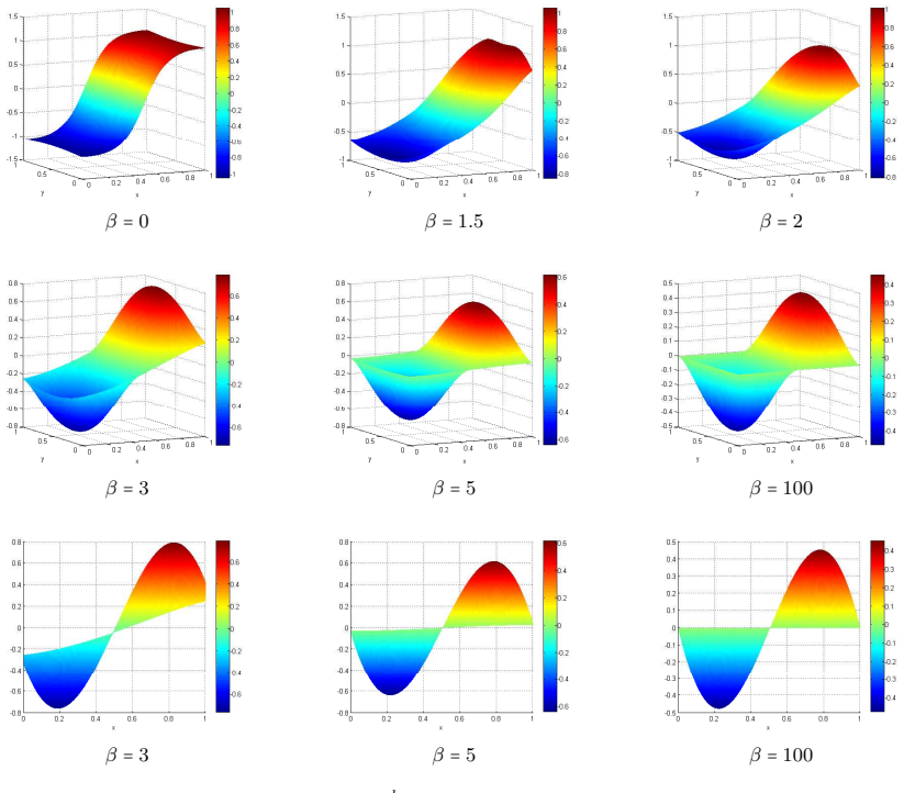
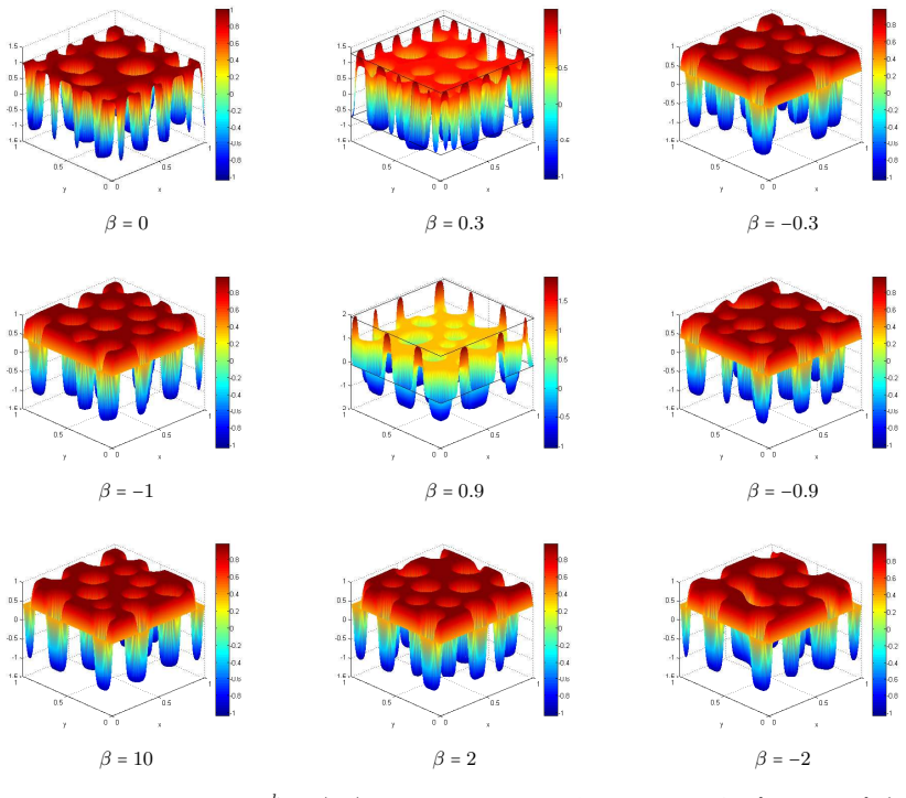
The extended model allows the surface and bulk order parameters to be opposite, as with $\alpha=-1$, producing solutions such as $(u,v)=(\pm 1,\mp 1)$ that are impossible in the original model where $u=v$ on the boundary.
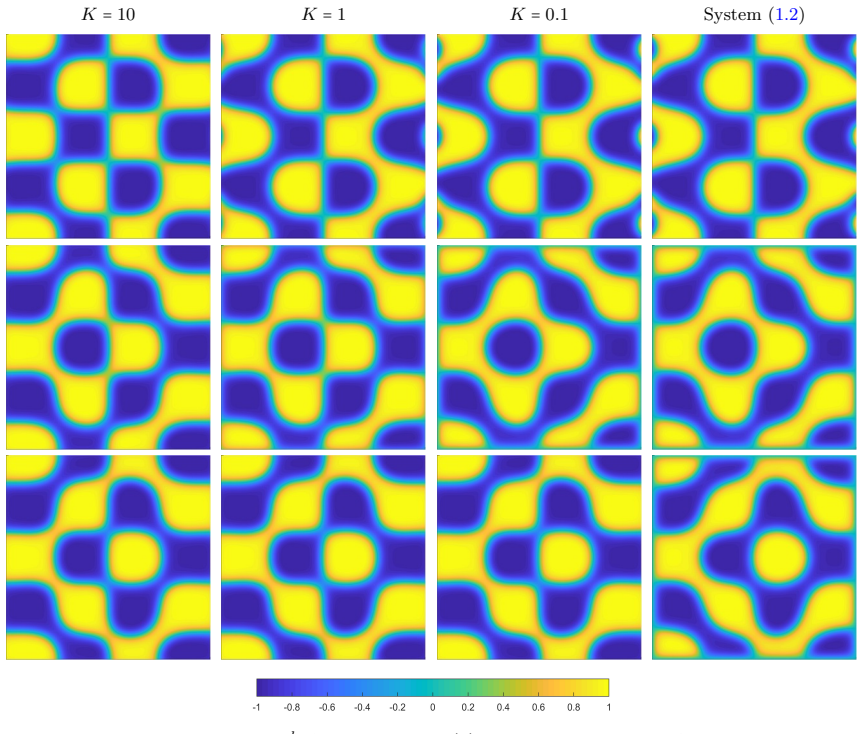
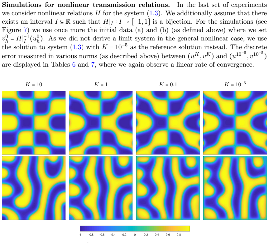
The numerical experiments show the same first-order behaviour for nonlinear relations such as $H(s)=\sin s$ and $H(s)=3\cos s+2$, suggesting that the affine-linear theory is the first instance of a wider principle.
In the absence of surface diffusion ($\kappa=0$), existence, uniqueness, and convergence still hold, but the error estimate loses the surface $H^1$ and $L^4$-in-time bounds and requires a convex surface potential with $G_2\equiv 0$.

Reading between the lines

Editorial extensions of the paper, not claims the author makes directly.

If the linear-rate convergence observed for nonlinear $H$ can be proved under assumptions that replace the affine structure, the Robin regularisation would become a general numerical route to nonlinear dynamic boundary conditions; a natural first target is monotone $H$ with controlled growth, where Minty's trick might replace the affine structure.
The error bound's dependence on $\|\partial_\nu u\|$ suggests that convergence will slow down when the limit solution develops steep boundary layers, making an adaptive choice of $K$ tied to the local normal-derivative size a testable extension.
The numerical competition between boundary mass conservation and phase separation suggests a predictive criterion based on whether the boundary mean lies between the stable minima of the shifted surface potential $G(\alpha^{-1}(s-\beta))$; the authors report explicit counterexamples, so a refined criterion involving profile shape or parameter ratios is still open.
The same gradient-flow discretisation used for existence can likely be turned into a structure-preserving scheme; proving convergence of the fully discrete scheme as the mesh size and time step go to zero simultaneously with $K$ would make the numerical proxy fully rigorous.

Share X Bluesky LinkedIn Reddit HN

Signed reviews

No signed human review yet.

Editorial analysis

A structured set of objections, weighed in public.

Desk editor's note, referee report, and a circularity audit.

Desk Editor's Note

read the letter

Dear colleague,

Read Knopf-Lam on the Robin boundary approximation for the Liu-Wu Cahn-Hilliard system. Short version: this is a competent extension paper, and the central convergence claim is real but narrower than the abstract makes it sound. The genuinely new pieces are the affine-linear transmission condition u=αv+β and the proof that Robin regularization converges to the extended system, with an O(K) error bound in the affine case. The κ=0 no-surface-diffusion regime is also treated, and that is where the interesting restrictions live.

What the paper does well: existence and uniqueness for both the limit and Robin systems are built on a natural gradient-flow structure, and the proofs are mostly clean. Theorem 2.3 is derived honestly: the error depends on ∂_nu∈L2 and the initial-data mismatch, and the K-rate is linear. The numerical experiments are detailed, with EOC tables for several parameter choices and two nonlinear H; they support the affine theorem and give suggestive evidence for the nonlinear case. No code or data is included, but for an analysis paper that is a minor omission, not a real defect.

Soft spots, in order of importance. First, the κ=0 case is less general than the abstract implies. Theorem 2.3 for κ=0 requires B1: G2≡0 and G1'' of polynomial growth, plus the extra regularity condition (2.6) with |G1''| bounded for the error estimate. The standard quartic double-well potential cannot be decomposed that way with G2≡0 and G1 convex. So for the no-surface-diffusion case with the usual nonconvex surface energy, the paper proves only weak convergence under restrictive assumptions, and the O(K) proxy result is not established. The authors state these assumptions openly, so it is not a hidden flaw, but it should be flagged in the abstract and conclusion if the paper is revised.

Second, several load-bearing compactness and limit steps in Sections 4 and 5 are deferred to [19] and [8] with phrases like "we omit the details." That is acceptable when the analogy is exact, and here it mostly is, but a referee should confirm those citations carry the weight.

Third, the numerical section observes O(K) for nonlinear H, while the analysis only covers existence in that regime. The text is careful not to claim a theorem there, so this is just an honest observation.

Overall, the theorems are internally consistent, the citations are to independent published results, and the paper is upfront about its restrictions. It deserves serious refereeing. If it were mine, I would ask the authors to state the κ=0 convexity restriction in the abstract and to expand the deferred arguments where they are load-bearing.

Referee Report

0 major / 6 minor

Summary. The paper analyzes a Cahn–Hilliard system with a dynamic boundary condition, extending the Liu–Wu model by allowing an affine transmission relation u=αv+β on the boundary. The main results are: (i) Theorem 2.1, global existence and uniqueness of weak solutions to the extended limit system (1.1)–(1.2), including the no-surface-diffusion case κ=0; (ii) Theorem 2.2, global existence and uniqueness for the Robin-penalized system (1.3) under assumptions (A1)–(A3), with additional restrictions (B1)–(B2) in the case κ=0; and (iii) Theorem 2.3, weak convergence as K→0 and an explicit O(K) error estimate for affine H, under the additional regularity hypothesis (2.6). The proofs use the gradient-flow structure of both systems and an implicit time discretization, following the framework of [19], with a Minty-trick argument for the κ=0 surface potential and elliptic regularity estimates for the boundary normal derivative. The paper also presents finite-element simulations that show linear experimental order of convergence for affine relations and for two nonlinear relations.

Significance. If the results are correct, they provide a rigorous justification for using the Robin problem (1.3) as a numerical proxy for the dynamic boundary condition in the affine case, with a quantified rate. The treatment of κ=0 is a genuine extension of previous work and the restriction to convex surface potentials with G2≡0 is stated transparently in the theorem hypotheses. The paper is built on standard compactness and elliptic-regularity arguments, and the main theorems are internally consistent; no parameter fitting is involved. The numerical experiments are consistent with the theoretical rate, although they only cover κ>0 and no code is supplied. The main caveat is that the quantitative O(K) result in the no-surface-diffusion case does not cover the standard quartic double-well potential; this should be flagged prominently so that the scope of the headline claim is not overstated.

minor comments (6)

[Theorem 2.3, Section 2] In the convergence statement of Theorem 2.3, the line “µK⇀µ in L2(0,T;H1(Γ))” should read L2(0,T;H1(Ω)), since µ is the bulk chemical potential; the surface limit is correctly stated for αµKΓ.
[Abstract and Section 8] The abstract and conclusion state that the error estimate covers the no-surface-diffusion case, but for κ=0 the estimate is proved only under (B1) and (2.6), which require G2≡0 and |G1′′| bounded. These assumptions exclude the standard quartic double-well potential G(s)=1/4(s2−1)2, for which the natural decomposition has G2(s)=−s2/2+1/4 and G1′′(s)=3s2. Please state this restriction explicitly in the abstract and conclusion so that the scope of the O(K) claim is unambiguous.
[Section 5, Step 5] The convergence assertions for the time-discrete approximations are delegated to [19, Lem. 8] with the statement that the proof is “almost analogous.” For κ=0 the compactness of vN in C([0,T];H1(Γ)′) and the absence of strong convergence in L2(ΣT) are new features that are not present in [19]; please provide a self-contained argument or at least spell out the compact embedding and the equicontinuity steps used in this case.
[Section 7] All numerical experiments for the convergence as K→0 are performed with κ>0 (κ=1 or κ=0.4), so the numerically observed O(K) rate is not evidence for the analytically harder κ=0 case. A sentence acknowledging this and explaining whether the κ=0 regime is numerically accessible with the stated assumptions would be helpful.
[Section 7.1] The numerical implementation is described only through references to earlier work and MATLAB code; no code or data are provided. Please include a reproducibility statement or make the code available, since the convergence tables are otherwise difficult to verify independently.
[Section 4, Step 2] The uniform estimates in Step 2 are imported from [19] with the phrase “immediately infer.” Because the new affine transmission condition changes the boundary coupling and the κ=0 case changes the surface regularity, please specify exactly which estimates from [19] are being used and why the modifications do not affect them.

Circularity Check

0 steps flagged · score 0.0 of 10

No circularity: the Robin-to-Liu–Wu convergence is a proven theorem with independent citations, not a fit or a self-referential construction.

full rationale

The paper's main claims are theorems established by compactness, monotonicity, and Gronwall arguments; no parameter is fitted to data, and no target claim is used as an assumption. The Robin penalization (1.3) formally enforces u=H(v) as K→0 through the energy term (1/(2K))∫|H(v)−u|²dΓ, but Theorem 2.3 does not stop at this formal observation: it proves weak convergence of the full solution tuple and derives the quantitative bound (2.14) from the PDE system. The error bound's right-hand side contains ||∂n u||²_{L²(Σ_T)}, the normal derivative of the limit solution, which is a regularity hypothesis (2.6), not a fitted quantity or a restatement of the conclusion. Citations to [19] and [8] are used as proof scaffolding (implicit time discretization, elliptic regularity), but both are independent published works with their own proofs; the authors also supply enough of the adapted arguments in Sections 4–6 to make the dependency transparent. The restrictive assumptions (B1)–(B2) for κ=0 are mathematical hypotheses delimiting the proven regime, not circularity. Numerical experiments for nonlinear H are explicitly presented as observations, not theorems. Hence no circular step is present.

Assumptions & free parameters 0 free parameters · 8 assumptions · 0 invented entities

No parameters are fitted to data; the model constants (α,β,ε,δ,κ) are inputs, and the numerical choices in Section 7 are illustrative. The central claims are theorems conditional on explicitly stated assumptions. The only introduced object is the Robin penalty parameter K, a standard regularization device, not a new physical entity.

assumptions (8)

domain assumption Assumption (A1): Ω ⊂ R^d with d∈{2,3} is bounded with Lipschitz boundary Γ.
Sets the functional framework for Sobolev spaces and trace theorems throughout Sections 2-6.
domain assumption Assumption (A2): F and G are bounded below and split into convex F1,G1 and Lipschitz F2,G2.
Enables the convex-splitting implicit time discretization and the a priori estimates in Sections 4-5.
domain assumption Assumption (A3): H ∈ C^2(R) with polynomial growth bounds on H, H' and H''.
Controls the nonlinear Robin coupling terms in the regularized system.
domain assumption Condition (2.6): growth bounds on F'1 and G''1.
Ensures H^2 regularity of u and the trace regularity ∂nu∈L2(ΣT) needed for the error estimate.
domain assumption Assumption (B1): for κ=0, G2≡0 and G1 convex with polynomial growth of G1''.
Provides monotonicity and compactness for the no-surface-diffusion case, enabling Minty's trick.
domain assumption Assumption (B2): H(s)=αs+β for the convergence theorem.
The convergence result is proven only for affine linear H; nonlinear H is left for future work.
domain assumption Smooth boundary Γ for the error estimate (Remark 2.2).
Invoked for classical elliptic regularity results used in Theorem 2.3.
standard math Standard functional-analytic tools (solution operators N, NΓ, trace inequalities, Sobolev embeddings, Gronwall).
Background results listed as (P1)-(P6) and used across all proofs.

how reviews work

0 comments

Cite this review

Pith. "Pith review of Convergence of a Robin boundary approximation for a Cahn--Hilliard system with dynamic boundary conditions." pith.science (2026). https://pith.science/paper/DEEJYLCY

@misc{pith2026190806124,
  author       = {Pith},
  title        = {Pith review of: Convergence of a Robin boundary approximation for a Cahn--Hilliard system with dynamic boundary conditions},
  year         = {2026},
  howpublished = {\url{https://pith.science/paper/DEEJYLCY}},
  note         = {Machine review of arXiv:1908.06124}
}

read the original abstract

We prove the existence of unique weak solutions to an extension of a Cahn--Hilliard model proposed recently by C.~Liu and H.~Wu (2019), in which the new dynamic boundary condition is further generalised with an affine linear relation between the surface and bulk order parameters. As a first approach to tackle more general and nonlinear relations, we investigate the existence of unique weak solutions to a regularisation by a Robin boundary condition. Included in our analysis is the case where there is no diffusion for the surface order parameter, which causes new difficulties for the analysis of the Robin system. Furthermore, for the case of affine linear relations, we show the weak convergence of solutions as the regularisation parameter tends to zero, and derive an error estimate between the two models. This is supported by numerical experiments which also demonstrate some non-trivial dynamics for the extended Liu--Wu model that is not present in the original model.

Figures

Figures reproduced from arXiv: 1908.06124 by the authors.

**Figure 2.** Profiles of the discrete solution u k h to (1.1) at iteration k = 200 for α = 1 and β ∈ {0, 1.5, 2} (top row) and β ∈ {3, 5, 100} (middle row) all viewed in the same camera line of sight. (Bottom row) Profiles of the discrete solution for β ∈ {3, 5, 100} with a different camera line of sight. Note that the range of the z-axis can be different with each plot. conservation of boundary mass (∣Γ∣ ⟨u0⟩Γ = 1.606 to three … view at source ↗

**Figure 3.** Discrete solution u k h to (1.1) at iteration k = 200 for α = 1 and β ∈ {0, 0.3,−0.3} (top row) and β ∈ {−1, 0.9,−0.9} (middle row) and β ∈ {10, 2,−2} (bottom row). The two black level lines in the plot for β = 0.3 are {z = 1.3} and {z = −0.7}, and the two black level lines in the plot for β = 0.9 are {z = 1.9} and {z = −0.1}. ⟨u0⟩Γ ∈ (s1, s2) in each of these cases. Therefore, at present we do not have a robust met… view at source ↗

Figures from the paper (4 more)

**Figure 4.** Figure 4: Discrete initial data u 0 h in the cases (a) (left) and (b) (right). In Tables 1 to 5, we collect the error between the discrete solution (u K, vK) to (1.3) and the discrete solution (u, v) to (1.2) (where v stands for α −1 (u−β)) measured in various norms for several …

**Figure 5.** Figure 5: Numerical solution u k h for initial data (a) at iteration k = 100 for κ = 1 as well as (α, β) = (1, 0) (first row), (α, β) = (2,−4) (second row) and (α, β) = (−2, 4) (third row). K L 2 (H1 (Ω)) EOC L 4 (L 2 (Ω)) EOC L 2 (ΣT ) EOC 10 2.63e − 01 - 3.98e − 02 - 4.71e − 0…

**Figure 6.** Figure 6: Numerical solution u k h with initial data (b) at iteration k = 100 for κ = 0.4 as well as (α, β) = (1, 0) (first row), (α, β) = (2,−4) (second row) and (α, β) = (−5, 30) (third row). K L 2 (H1 (Ω)) EOC L 4 (L 2 (Ω)) EOC L 2 (ΣT ) EOC 10 2.66e − 01 - 3.73e − 02 - 4.99e…

**Figure 7.** Figure 7: ) we use once more the initial data (a) and (b) (as defined above) where we set v 0 h = H∣ −1 I (u 0 h ). As we did not derive a limit system in the general nonlinear case, we use the solution to system (1.3) with K = 10−5 as the reference solution instead. The discret…

Discussion (0). Continue with ORCID to comment.

Reference graph

Works this paper leans on

31 extracted references · 31 canonical work pages

[19]

Garcke and P

H. Garcke and P. Knopf. Weak solutions of the Cahn–Hilliard system with dynamic boundary con- ditions: A gradient ﬂow approach. SIAM J. Math. Anal. 52 (2020) 340–369

work page 2020
[8]

Colli, T

P. Colli, T. Fukao and K.F. Lam. On a coupled bulk-surface Allen–Cahn system with an aﬃne linear transmission condition and its approximation by a Robin boundary condition. Nonlinear Anal. 184 (2019) 116–147

work page 2019
[1]

H.W. Alt. Linear Functional Analysis - An Application-Oriented Introduction. Springer-Verlag Lon- don, 2016

work page 2016
[2]

A. Buﬀa, M. Costabel and D. Sheen. On traces for H(curl,Ω) in Lipschitz domains. J. Math. Anal. Appl. 276 (2002) 845–867

work page 2002
[3]

Calatroni and P

L. Calatroni and P. Colli. Global solution to the Allen-Cahn equation with singular potentials and dynamic boundary conditions. Nonlinear Anal. 79 (2013) 12–27

work page 2013
[4]

Cherﬁls, S

L. Cherﬁls, S. Gatti and A. Miranville. A variational approach to a Cahn–Hilliard model in a domain with nonpermeable walls. J. Math. Sci. 189 (2013) 604–636

work page 2013
[5]

Cherﬁls and M

L. Cherﬁls and M. Petcu. A numerical analysis of the Cahn–Hilliard equation with non-permeable walls. Numer. Math. 128 (2014) 517–549

work page 2014
[6]

Cherﬁls, M

L. Cherﬁls, M. Petcu and M. Pierre. A numerical analysis of the Cahn–Hilliard equation with dynamic boundary conditions. Discrete Contin. Dyn. Syst. 27 (2010) 1511–1533

work page 2010

Show all 31 references

[7]

Colli and T

P. Colli and T. Fukao. Equation and dynamic boundary condition of Cahn–Hilliard type with singular potentials. Nonlinear Anal. 127 (2015) 413–433

2015
[9]

Colli, T

P. Colli, T. Fukao and H. Wu. On a transmission problem for equation and dynamic boundary condition of Cahn–Hilliard type with nonsmooth potentials. arXiv:1907.13279 [math.AP] (2019)

2019 arXiv
[10]

L.C. Evans. Partial Diﬀerential Equations. AMS, Providence, R.I. 2010

2010
[11]

Feng and A

X. Feng and A. Prohl. Error analysis of a mixed ﬁnite element method for the Cahn–Hilliard equation. Numer. Math. 99 (2004) 47–84

2004
[12]

Feng and A

X. Feng and A. Prohl. Numerical analysis of the Cahn–Hilliard equation and approximation for the Hele-Shaw problem. Interfaces Free Bound. 7 (2005) 1–28 40

2005
[13]

Fischer, P

H.P. Fischer, P. Maass and W. Dieterich. Novel surface modes in spinodal decomposition. Phys. Rev. Lett. 79 (1997) 893–896

1997
[14]

Fischer, J

H.P. Fischer, J. Reinhard, W. Dieterich, J.-F. Gouyet, P. Maass, A. Majhofer and D. Reinel. Time- dependent density functional theory and the kinetics of lattice gas systems in contact with a wall. J. Chem. Phys. 108 (1998) 3028–3037

1998
[15]

Fukao, S

T. Fukao, S. Yoshikawa and S. Wada. Structure-preserving ﬁnite diﬀerence schemes for the Cahn– Hilliard equation with dynamic boundary conditions in the one-dimensional case. Commun. Pure Applied Anal. 16 (2017) 1915–1938

2017
[16]

C.G. Gal, M. Grasselli and A. Miranville. Cahn–Hilliard–Navier–Stokes systems with moving contact lines. Calc. Var. Partial Diﬀer. Equ. 55 (2016) article 50

2016
[17]

C.G. Gal, M. Grasselli and H. Wu. Global weak solutions to a diﬀuse interface model for incompress- ible two-phase ﬂows with moving contact lines and diﬀerent densities. Arch. Rational Mech. Anal. 234 (2019) 1–56

2019
[18]

Garcke, On Cahn–Hilliard systems with elasticity

H. Garcke, On Cahn–Hilliard systems with elasticity. Proc. Roy. Soc. Edinburgh 133 A (2003), pp. 307–331

2003
[20]

Goldstein, A

G.R. Goldstein, A. Miranville and G. Schimperna. A Cahn–Hilliard model in a domain with non- permeable walls. Phys. D 240 (2011) 754–766

2011
[21]

Guill´ en-Gonz´ alez and G

F. Guill´ en-Gonz´ alez and G. Tierra. On linear schemes for a Cahn–Hilliard diﬀuse interface model. J. Comput. Phys. 243 (2013) 140–171

2013
[22]

Israel, A

H. Israel, A. Miranville and M. Petcu. Numerical analysis of a Cahn–Hilliard type equation with dynamic boundary conditions. Ricerche Mat. 64 (2015) 25–50

2015
[23]

Kenzler, F

R. Kenzler, F. Eurich, P. Maass, B. Rinn, J. Schropp, E. Bohl and W. Dieterich. Phase separation in conﬁned geometries: solving the Cahn–Hilliard equation with generic boundary conditions. Comput. Phys. Commun. 133 (2001) 139–157

2001
[24]

Kov´ acs and C

B. Kov´ acs and C. Lubich. Numerical analysis of parabolic problems with dynamic boundary condi- tions. IAM J. Numer. Anal. 37 (2017) 1–39

2017
[25]

Liu and H

C. Liu and H. Wu. An Energetic Variational Approach for the Cahn–Hilliard Equation with Dynamic Boundary Conditions: Model Derivation and Mathematical Analysis. Arch. Rational Mech. Anal. 233 (2019) 167–247

2019
[26]

S. Metzger. An eﬃcient and convergent ﬁnite element scheme for Cahn–Hilliard equations with dynamic boundary conditions. arXiv:1908.04910 [math.NA] (2019)

2019 arXiv
[27]

Miranville

A. Miranville. The Cahn–Hilliard Equation: Recent Advances and Applications. CBMS-NSF Re- gional Conference Series in Applied Mathematics. SIAM 2019

2019
[28]

Qian, X.P

T.Z. Qian, X.P. Wang and P. Sheng. A variational approach to moving contact line hydrodynamics. J. Fluid Mech. 564 (2006) 333–360

2006
[29]

J. Shen, J. Xu and J. Yang. The scalar auxiliary variable (SAV) approach for gradient ﬂows. J. Comput. Phys. 353 (2018) 407–416

2018
[30]

Shen and X

J. Shen and X. Yang. Numerical approximation of Allen-Cahn and Cahn-Hilliard equations. Discrete Contin. Dyn. Syst. 28 (2010) 1669–1691

2010
[31]

Trautwein

D. Trautwein. Finite-Elemente Approximation der Cahn-Hilliard-Gleichung mit Neumann- und dy- namischen Randbedingungen. Bachelor thesis, University of Regensburg (2018) 41

2018

Pith tools

Reviewed August 14, 2026 · model on record in the stance chip above.

[1] [19]

Garcke and P

H. Garcke and P. Knopf. Weak solutions of the Cahn–Hilliard system with dynamic boundary con- ditions: A gradient ﬂow approach. SIAM J. Math. Anal. 52 (2020) 340–369

work page 2020

[2] [8]

Colli, T

P. Colli, T. Fukao and K.F. Lam. On a coupled bulk-surface Allen–Cahn system with an aﬃne linear transmission condition and its approximation by a Robin boundary condition. Nonlinear Anal. 184 (2019) 116–147

work page 2019

[3] [1]

H.W. Alt. Linear Functional Analysis - An Application-Oriented Introduction. Springer-Verlag Lon- don, 2016

work page 2016

[4] [2]

A. Buﬀa, M. Costabel and D. Sheen. On traces for H(curl,Ω) in Lipschitz domains. J. Math. Anal. Appl. 276 (2002) 845–867

work page 2002

[5] [3]

Calatroni and P

L. Calatroni and P. Colli. Global solution to the Allen-Cahn equation with singular potentials and dynamic boundary conditions. Nonlinear Anal. 79 (2013) 12–27

work page 2013

[6] [4]

Cherﬁls, S

L. Cherﬁls, S. Gatti and A. Miranville. A variational approach to a Cahn–Hilliard model in a domain with nonpermeable walls. J. Math. Sci. 189 (2013) 604–636

work page 2013

[7] [5]

Cherﬁls and M

L. Cherﬁls and M. Petcu. A numerical analysis of the Cahn–Hilliard equation with non-permeable walls. Numer. Math. 128 (2014) 517–549

work page 2014

[8] [6]

Cherﬁls, M

L. Cherﬁls, M. Petcu and M. Pierre. A numerical analysis of the Cahn–Hilliard equation with dynamic boundary conditions. Discrete Contin. Dyn. Syst. 27 (2010) 1511–1533

work page 2010