REVIEW 3 major objections 4 minor 159 references
Simulation and Learning for Urban Mobility: City-scale Traffic Reconstruction and Autonomous Driving
T0 review · 3 major / 4 minor · reviewed 2026-08-14 · deepseek-v4-flash
Pith's one-line read The paper claims that sparse GPS data can reconstruct city-scale traffic when map matching follows shortest travel time rather than shortest distance, and that simulated accidents can supply training data for effective autonomous driving.
desk verdict A capable dissertation that compiles the author's own published work on traffic reconstruction and learning-based driving, with a real soft spot: the headline synthetic evaluations assume exactly the route-choice criterion the method depends on. read the letter →
The pith
A machine-rendered reading of the paper's core claim, the machinery that carries it, and where it could break.
The reading
What carries the argument
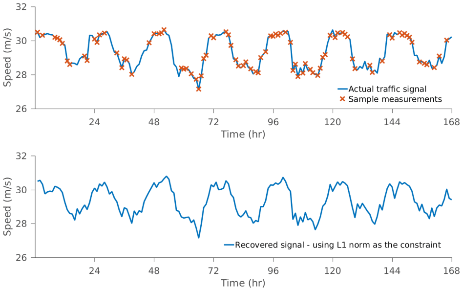
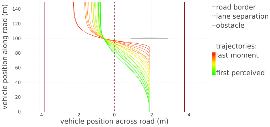
The reconstruction pipeline's load-bearing object is the relaxation algorithm: for each pair of consecutive GPS points it extracts a sub-network, finds candidate fastest paths, and repeatedly slows down road segments on overestimated paths until every candidate path's travel time equals the timestamp difference, an operation whose correctness rests on Wardrop's user-equilibrium assumption that all traces are fastest routes. Travel-time allocation along each path uses a decomposition into free-flow, congestion, and stopping times adapted from Hellinga et al., and the monotone decrease of speeds (Theorem 2.1) keeps the search efficient. Temporal missing data are handled by treating the weekly speed pattern of a road segment as a sparse signal in the DCT domain and recovering it by $\ell^1$-minimization, a compressed-sensing step that needs about 90 measurements instead of 168. Spatial missing data are completed by a trust-region optimization over intersection turning ratios, using a metamodel that blends a physical flow-conservation model with a quadratic polynomial so simulated flows obey the boundary flows estimated from GPS data. The driving side is carried by SimExpert, the simulated expert that plans many alternative safe trajectories for a vehicle after an accident and assigns DANGER/SAFE labels to states, automatically generating the heterogeneous training set for the hierarchical LSTM policy.
What would settle it
Give the algorithm a congested urban network with known ground-truth travel times and a set of GPS traces whose true routes are known from high-frequency onboard logging. If a substantial fraction of traces follow routes that are not the fastest available (shortest-distance or habitual choices), the recovered travel times should be compared against the ground truth: the central claim would fail if the mean absolute error grows to the level of the shortest-distance baseline or worse as the fraction of non-fastest traces increases. A simpler probe: on such a dataset, check whether the relaxation's inferred network speeds are systematically higher on routes that the fastest-path assumption actually penalizes.
Extended reading notes
Core claim
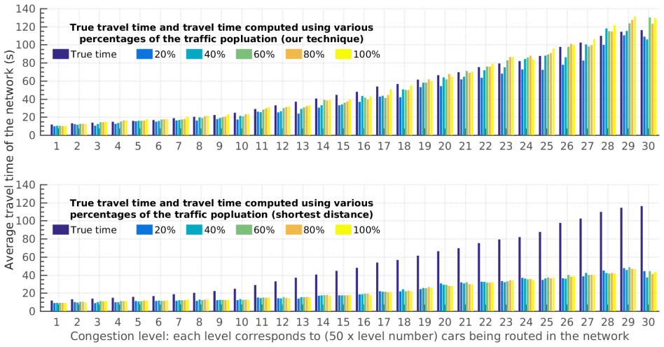
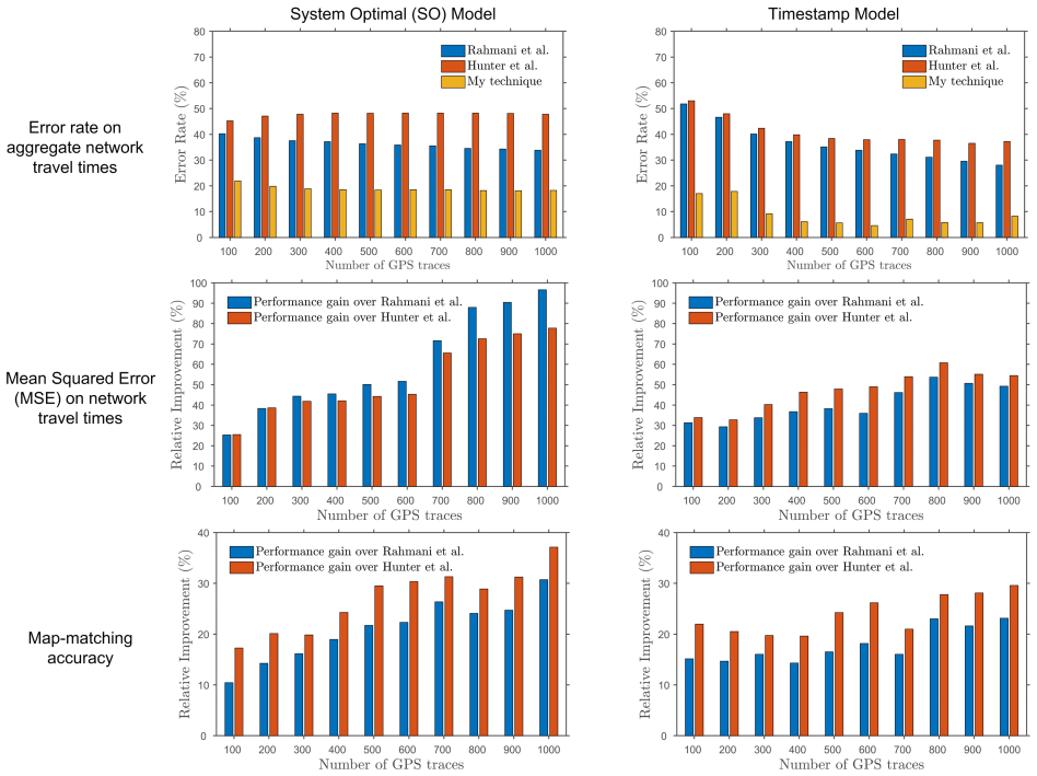
The central claim is that the speed of every road segment in a city can be recovered from GPS traces that are sparse in space and time, provided map matching uses estimated shortest travel times rather than shortest distances. Starting from a network at free-flow speed, the relaxation algorithm takes each trace's timestamp difference as the true travel time of the fastest path, and repeatedly increases travel times on overestimated candidate paths until they match it; because road-segment speeds only decrease during this process, the procedure is tractable and terminates. The dissertation reports that this approach, followed by compressed-sensing completion of missing time intervals and metamodel-driven flow completion for uncovered areas, reconstructs travel times with mean absolute error of $3.40$ s (std. $3.32$) at 80% trace penetration, versus $29.55$ s (std. $22.46$) for a shortest-distance baseline, and yields up to 97% relative mean-squared-error improvement over two state-of-the-art travel-time estimators. For autonomous driving, the paper claims that a 2D simulated expert which plans alternative safe trajectories under kinematic and dynamic constraints can turn a simulated accident into a large set of labeled recovery examples, and that a hierarchical detection/following/avoidance policy trained on these examples avoids obstacles in on-road and off-road scenarios where an end-to-end baseline fails. The theoretical guarantee bounds the learned policy's cost-to-go by $J(\hat{\pi})\le T\hat{\epsilon}_{\min}+T\hat{\epsilon}_{\mathrm{regret}}+O(Tl_{\max}\sqrt{\log(1/\mu)/(KN)})$.
Load-bearing premise
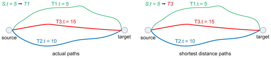
The framework assumes that every GPS trace follows the fastest path under the true traffic conditions, so the observed timestamp difference is the minimum travel time between the two GPS points; if drivers frequently take shortest-distance or habitual routes instead, the relaxation will systematically distort the reconstructed travel times.
Editorial extensions
If this is right
- Citywide traffic monitoring becomes possible from low-penetration GPS fleets: the reported mean travel-time error stays between about $3.4$ and $8.3$ s across 20% to 100% trace penetration, far below the shortest-distance baseline.
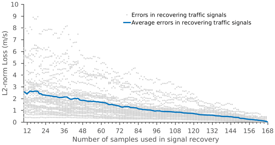
- Temporal gaps in GPS coverage can be filled by exploiting weekly periodicity: compressed sensing recovers a traffic signal with roughly 90 measurements, about half of what the Nyquist rate requires, and error grows only linearly as samples decrease.
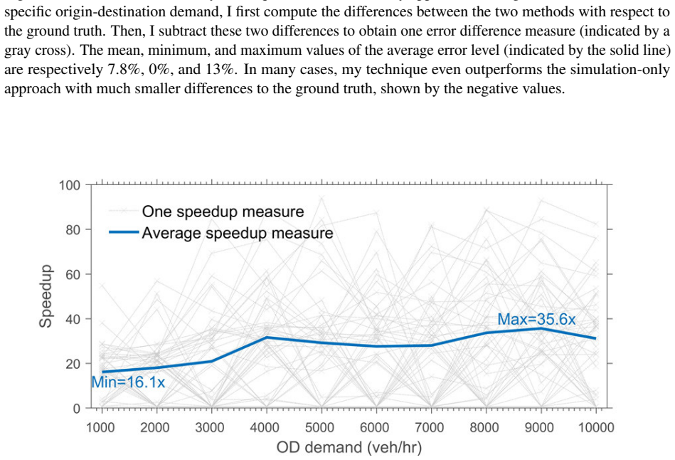
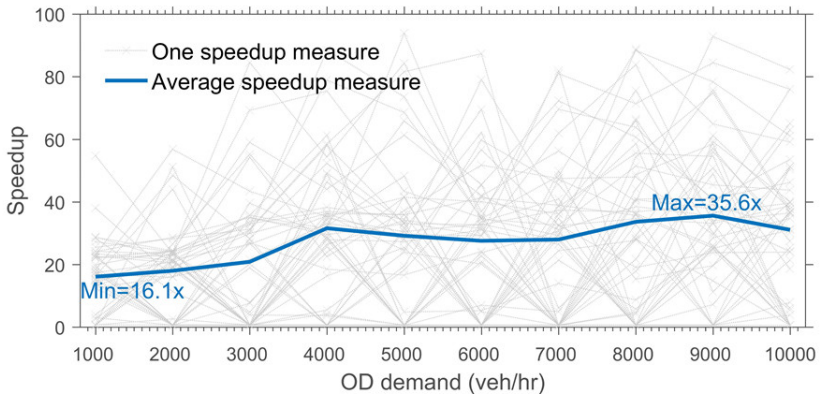
- Areas without GPS coverage can be reconstructed by tuning simulation turning ratios with a metamodel, achieving roughly 27x average speedup over a simulation-only approach while keeping about 7.8% average error on the tested networks.
- A single simulated accident can generate a large, heterogeneous batch of labeled recovery trajectories, and the ADAPS bound shows the policy cost converges to $T\hat{\epsilon}_{\min}+O(\epsilon)$ once $O(T^2l_{\max}^2\log(1/\mu)/\epsilon^2)$ examples are collected.
- The hierarchical detect-follow-avoid policy trained this way reaches 100% success in 50-run tests on straight and curved roads with a static obstacle, while the compared end-to-end policy fails in both cases.
Reading between the lines
- The reliance on a single routing criterion is the most exposed point; a natural extension is to model drivers as choosing among several criteria (fastest, shortest, habitual) and estimate the mixing proportions jointly with travel times, which the relaxation machinery could support without changing its core loop.
- The compressed-sensing component transfers beyond traffic: any periodic spatiotemporal field with a few dominant frequencies and sparse mobile measurements could be completed by the same $\ell^1$-recovery scheme, provided the coherence condition holds.
- The ADAPS theoretical guarantee presumes the simulation can place the agent in arbitrary states; physical deployment would likely require bridging the sim-to-real gap through domain randomization or fine-tuning, which the dissertation does not address.
- The 27x speedup reported for metamodel-based completion points toward real-time traffic reconstruction and interactive urban visualization, but the dissertation does not demonstrate real-time update rates.
Signed reviews
Editorial analysis
A structured set of objections, weighed in public.
Referee Report
Summary. This dissertation presents a two-part framework for urban mobility. The first part addresses city-scale traffic reconstruction from sparse GPS traces, proposing a shortest-travel-time map-matching and relaxation algorithm, a compressed-sensing method for temporal missing data, an iterative estimation procedure, and a metamodel-based simulation optimization for spatial completion. The second part proposes ADAPS, a simulation-based framework for learning autonomous driving policies from accident recovery demonstrations, with a hierarchical control policy and a DAGGER-style theoretical guarantee. The traffic reconstruction is evaluated against Lou et al., Hunter et al., and Rahmani et al. on synthetic GPS traces and on the Cabspotting dataset; the ADAPS policy is tested in straight-road, curved-road, and open-ground simulated scenarios. The central quantitative claims are that the proposed methods yield consistently lower travel-time estimation errors and robust collision avoidance.
Significance. The dissertation addresses an important problem with a principled approach: replacing shortest-distance map matching by shortest travel-time matching is well motivated by Wardrop's user equilibrium, and the relaxation algorithm is an original way to exploit the lower-bound structure. The compressed-sensing analysis of traffic signal sparsity is solid, and the metamodel-based simulation optimization is an interesting contribution for spatial completion. For autonomous driving, using simulated accidents to generate recovery data is a creative and potentially impactful idea, and the theoretical bound in Theorem 1.1 transfers the DAGGER-style guarantee to a generative setting. The experimental work is extensive, and the dissertation includes formal statements (Theorem 2.1, Corollaries 2–3, Theorem 1.1) that are clearly derived. However, as detailed in the major comments, the evaluation of the traffic reconstruction is self-consistent rather than probative for real-world route choice, which limits the strength of the headline claims.
major comments (3)
- [§2.3.2, §2.3.4, §3.6.1.4] The central evaluation of the traffic reconstruction is performed on synthetic GPS traces generated with the same routing rule that the method assumes: Assumption 1 (§2.3.2) states that all GPS traces are planned using the shortest travel-time criterion, and §2.3.4 states that 'All traces are simulated by randomly selecting nodes... using the fastest route strategy'; §3.6.1.4 repeats this with 'routing with the shortest travel-time strategy.' Consequently, Tables 1.1/2.1 and Figures 3.4–3.7 demonstrate that the method works when the world obeys Assumption 1, but they do not test route-choice behaviors that violate it (e.g., shortest-distance or stochastic routes). Since the relaxation algorithm relies on the lower-bound property of Corollary 2, a mismatch between Assumption 1 and real driver behavior could systematically bias travel-time estimates and map-matched paths. The real-data evaluation (§2.5, §3.6.3) is qualitative: it shows recovered daily periodicity, day-to-day cosine similarities, and a roughly 1 m/s speed loss against three loop detectors after frequency filtering, but it does not validate road-segment-level travel-time accuracy or map-matching correctness. I recommend adding synthetic experiments with alternative route-choice models and, if possible, validating on real trajectories with known ground truth.
- [§2.4, Eqs. (2.8)–(2.10)] The compressed-sensing recovery is validated on loop-detector signals using random row-permutation sampling (§2.4: 'I test the performance of my method by first obtaining random measurements via sampling...'). However, the missingness in real GPS data is structured: some time intervals (e.g., early-morning hours) are systematically underrepresented, and the set of available hourly measurements per road segment is determined by traffic coverage rather than by a random process. The bound m_min = μ²S log(n) and the robustness result in Figure 2.10 are derived under random sampling conditions, so their validity for the GPS application is not established. I recommend testing the recovery under structured missing patterns (e.g., removing entire time blocks) or otherwise qualifying the claim that the minimum number of measurements for GPS-based recovery is 90.
- [§4.7, Table 4.2] The ADAPS evaluation is limited to three simple simulated scenarios (straight road, curved road, and open ground), and the success metric in Table 4.2 is the fraction of collision-free laps or obstacle-avoidance runs. The thesis statement (§1.4) claims 'robust control policies for autonomous driving,' but no experiments address unseen road geometries, varying traffic densities, sensor noise, or environmental variations (lighting, weather), nor is the learned policy compared with a DAGGER-trained policy in terms of cost-to-go or number of iterations. The theoretical bound in Theorem 1.1 is DAGGER-style and does not by itself establish robustness in the tested sense. The authors should either broaden the empirical validation or explicitly scope the robustness claim to the simulated test scenarios.
minor comments (4)
- [§2.3] There are several typos: 'noval' should be 'novel' in the first paragraph of Section 2.3, 'acutual' appears in Equation 3.28, and 'Collorary' is repeatedly used instead of 'Corollary' in Section 2.3.2.
- [§3.4.1] In the Wardrop constraints, the notation 't(s1,t 2)' should read 't(s1,s 2)' to denote the travel time between the two GPS points.
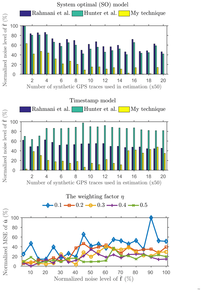
- [§2.3.3, Eq. (2.2)] The weighting factor β in the stopping likelihood function is set to 0.5 without a sensitivity analysis or justification; a brief study of the effect of β on travel-time allocation would strengthen the results.
- [§1.3.1.3] The introduction states 'up to 97% relative improvement' and 'up to 90 times speedup'; these claims are consistent with the figures, but the figure captions should identify the baselines (Hunter et al., Rahmani et al., simulation-only) more explicitly for the reader.
Circularity Check
No circular derivation found; synthetic evaluation is assumption-congruent but predicted quantities are not equivalent to inputs by construction.
full rationale
The derivation chain is not circular. Assumption 1 in Section 2.3.2 (\u201call GPS traces are planned using the shortest travel time criterion\u201d) is explicitly stated as a modeling assumption; it is not a conclusion derived from the target outputs. The map-matching and travel-time allocation procedures operate on GPS traces and allocate aggregate timestamp differences to road segments, and the resulting per-segment travel times are evaluated against ground-truth travel times from SUMO, the system-optimal model, the Timestamp model, and loop detectors. These external benchmarks are independent of the algorithm\u2019s fitted parameters, so the claimed improvements over Lou et al., Hunter et al., and Rahmani et al. are not forced by construction. \n\nThe compressed-sensing recovery (Section 2.4) estimates the sparsity level S from loop-detector signals and then uses S to compute the required number of measurements m_min before recovering the same type of signals via L1 minimization. This is a mild test-set dependence in choosing m_min, but the recovered signal is the solution of an underdetermined convex program and is not equal to the sparsity estimate; the reported errors (e.g., average error 1.4m/s) are measured on actual recovered signals, so this does not reduce the prediction to a fit. \n\nThe synthetic traces in Section 2.3.4 and Section 3.6.1.4 are generated under the same shortest-travel-time routing strategy that Assumption 1 posits. This makes the evaluation assumption-congruent and limits evidence about real-world route-choice behavior, but it does not make the output travel times a deterministic function of the input assumption; the relaxation and allocation procedures can still misestimate when routes or congestion differ. This is a validity limitation, not a circularity. \n\nThe ADAPS theoretical bound (Theorem 1.1, Section 1.3.2.1) is adapted from the DAGGER result of Ross et al. (2011) and is not imported from the author\u2019s own uniqueness theorems. The dissertation cites the author\u2019s earlier papers (Li et al. 2017a, 2017b, 2018, 2019), but those are published works providing prior support rather than load-bearing self-citations that replace independent verification. No equation or claim in the paper reduces by definition to its own inputs, so no circular step is established.
Assumptions & free parameters
free parameters (3)
- Beta (stopping likelihood weight) =
0.5
- Outer loop iterations =
10
- Sparsity level S for compressed sensing =
17.63
assumptions (4)
- domain assumption Assumption 1: All GPS traces are planned using the shortest travel-time criterion.
- domain assumption Wardrop's user equilibrium approximates real-world traffic
- domain assumption Surrogate loss l upper bounds the true cost C and is convex in the policy
- domain assumption Travel time distributions of road segments are pairwise independent and Gamma distributed
Cite this review
Pith. "Pith review of Simulation and Learning for Urban Mobility: City-scale Traffic Reconstruction and Autonomous Driving." pith.science (2026). https://pith.science/paper/IPWZI2HC
@misc{pith2026190806131,
  author       = {Pith},
  title        = {Pith review of: Simulation and Learning for Urban Mobility: City-scale Traffic Reconstruction and Autonomous Driving},
  year         = {2026},
  howpublished = {\url{https://pith.science/paper/IPWZI2HC}},
  note         = {Machine review of arXiv:1908.06131}
}
abstract
Traffic congestion has become one of the most critical issues worldwide. The costs due to traffic gridlock and jams are approximately $160 billion in the United States, more than {\pounds}13 billion in the United Kingdom, and over one trillion dollars across the globe annually. As more metropolitan areas will experience increasingly severe traffic conditions, the ability to analyze, understand, and improve traffic dynamics becomes critical. This dissertation is an effort towards achieving such an ability. I propose various techniques combining simulation and machine learning to tackle the problem of traffic from two perspectives: city-scale traffic reconstruction and autonomous driving.
Figures


Figures from the paper (43 more)

















Reference graph
Works this paper leans on
-
[1]
Abadi, A., Rajabioun, T., and Ioannou, P. A. (2015). Traffic flow prediction for road transportation networks with limited traffic data. IEEE Transactions on Intelligent Transportation Systems , 16(2):653--662
2015
-
[2]
Agarwal, S., Kachroo, P., and Contreras, S. (2016). A dynamic network modeling-based approach for traffic observability problem. IEEE Transactions on Intelligent Transportation Systems , 17(4):1168--1178
2016
-
[3]
Anava, O., Hazan, E., and Zeevi, A. (2015). Online time series prediction with missing data. In Proceedings of the 32nd International Conference on Machine Learning (ICML) , pages 2191--2199
2015
-
[4]
and Andrienko, G
Andrienko, N. and Andrienko, G. (2006). Exploratory analysis of spatial and temporal data: a systematic approach . Springer Science & Business Media
2006
-
[5]
T., Mitrovic, N., Dauwels, J., and Jaillet, P
Asif, M. T., Mitrovic, N., Dauwels, J., and Jaillet, P. (2016). Matrix and tensor based methods for missing data estimation in large traffic networks. IEEE Transactions on Intelligent Transportation Systems , 17(7):1816--1825
2016
-
[6]
Atkeson, C. G. (1994). Using local trajectory optimizers to speed up global optimization in dynamic programming. In Advances in neural information processing systems , pages 663--670
1994
-
[7]
G., Moore, A
Atkeson, C. G., Moore, A. W., and Schaal, S. (1997). Locally weighted learning. Artificial Intelligence Review , 11(1-5):11--73
1997
-
[8]
A., Kakade, S
Bagnell, J. A., Kakade, S. M., Schneider, J. G., and Ng, A. Y. (2004). Policy search by dynamic programming. In Advances in neural information processing systems , pages 831--838
2004
Show all 159 references
-
[9]
Barto, A. G. and Mahadevan, S. (2003). Recent advances in hierarchical reinforcement learning. Discrete Event Dynamic Systems , 13(4):341--379
2003
-
[10]
Bayarri, S., Fernandez, M., and Perez, M. (1996). Virtual reality for driving simulation. Commun. ACM , 39(5):72--76
1996
-
[11]
and Rao, K
Bera, S. and Rao, K. V. K. (2011). Estimation of origin-destination matrix from traffic counts: the state of the art. European Transport Trasporti Europei n. , pages 3--23
2011
-
[12]
Bi, H., Mao, T., Wang, Z., and Deng, Z. (2016). A data-driven model for lane-changing in traffic simulation. In Proceedings of the ACM SIGGRAPH/Eurographics Symposium on Computer Animation , pages 149--158
2016
-
[13]
D., Monfort, M., Muller, U., Zhang, J., et al
Bojarski, M., Del Testa, D., Dworakowski, D., Firner, B., Flepp, B., Goyal, P., Jackel, L. D., Monfort, M., Muller, U., Zhang, J., et al. (2016). End to end learning for self-driving cars. arXiv preprint arXiv:1604.07316
2016 arXiv
-
[14]
Candes, E., Romberg, J., and Tao, T. (2006). Robust uncertainty principles: exact signal reconstruction from highly incomplete frequency information. Information Theory, IEEE Transactions on , 52(2):489--509
2006
-
[15]
and Wakin, M
Cand \`e s, E. and Wakin, M. (2008). An introduction to compressive sampling. IEEE signal processing magazine , 25(2):21--30
2008
-
[16]
and Nguyen, S
Cascetta, E. and Nguyen, S. (1988). A unified framework for estimating or updating origin/destination matrices from traffic counts. Transportation Research Part B: Methodological , 22(6):437--455
1988
-
[17]
S., Zhang, D., and Li, S
Castro, P. S., Zhang, D., and Li, S. (2012). Urban traffic modelling and prediction using large scale taxi gps traces. In International Conference on Pervasive Computing , pages 57--72
2012
-
[18]
Celikoglu, H. B. (2007). A dynamic network loading model for traffic dynamics modeling. IEEE Transactions on Intelligent Transportation Systems , 8(4):575--583
2007
-
[19]
B., Gedizlioglu, E., and Dell'Orco, M
Celikoglu, H. B., Gedizlioglu, E., and Dell'Orco, M. (2009). A node-based modeling approach for the continuous dynamic network loading problem. IEEE Transactions on Intelligent Transportation Systems , 10(1):165--174
2009
-
[20]
Celikoglu, H. B. and Silgu, M. A. (2016). Extension of traffic flow pattern dynamic classification by a macroscopic model using multivariate clustering. Transportation Science , 50(3):966--981
2016
-
[21]
C., and Deng, Z
Chao, Q., Bi, H., Li, W., Mao, T., Wang, Z., Lin, M. C., and Deng, Z. (2019). A survey on visual traffic simulation: Models, evaluations, and applications in autonomous driving. Computer Graphics Forum
2019
-
[22]
Chao, Q., Deng, Z., Ren, J., Ye, Q., and Jin, X. (2018). Realistic data-driven traffic flow animation using texture synthesis. IEEE Transactions on Visualization and Computer Graphics , 24(2):1167--1178
2018
-
[23]
Chao, Q., Shen, J., and Jin, X. (2013). Video-based personalized traffic learning. Graphical Models , 75(6):305--317
2013
-
[24]
and Chrysanthou, Y
Charalambous, P. and Chrysanthou, Y. (2014). The pag crowd: A graph based approach for efficient data-driven crowd simulation. Computer Graphics Forum , 33(8):95--108
2014
-
[25]
Y., Yuan, H., Li, Q., Lam, W
Chen, B. Y., Yuan, H., Li, Q., Lam, W. H., Shaw, S.-L., and Yan, K. (2014). Map-matching algorithm for large-scale low-frequency floating car data. International Journal of Geographical Information Science , 28(1):22--38
2014
-
[26]
Chen, C., Seff, A., Kornhauser, A., and Xiao, J. (2015). Deepdriving: Learning affordance for direct perception in autonomous driving. In Computer Vision, 2015 IEEE International Conference on , pages 2722--2730
2015
-
[27]
Chen, G., Esch, G., Wonka, P., M \"u ller, P., and Zhang, E. (2008). Interactive procedural street modeling. ACM Trans. Graph. , 27(3):103:1--103:10
2008
-
[28]
Codevilla, F., M \"u ller, M., Dosovitskiy, A., L \'o pez, A., and Koltun, V. (2017). End-to-end driving via conditional imitation learning. In Robotics and Automation (ICRA), 2017 IEEE International Conference on , pages 746--753. IEEE
2017
-
[29]
Conn, A., Scheinberg, K., and Vicente, L. N. (2009). Introduction to derivative-free optimization , volume 8. SIAM
2009
-
[30]
Daum \'e , H., Langford, J., and Marcu, D. (2009). Search-based structured prediction. Machine learning , 75(3):297--325
2009
-
[31]
Donoho, D. (2006). Compressed sensing. Information Theory, IEEE Transactions on , 52(4):1289--1306
2006
-
[32]
and Egyh \'a ziov \'a , E
Faghri, A. and Egyh \'a ziov \'a , E. (1999). Development of a computer simulation model of mixed motor vehicle and bicycle traffic on an urban road network. Transportation research record , 1674(1):86--93
1999
-
[33]
T., Freire, J., and Silva, C
Ferreira, N., Poco, J., Vo, H. T., Freire, J., and Silva, C. T. (2013). Visual exploration of big spatio-temporal urban data: A study of new york city taxi trips. IEEE Transactions on Visualization and Computer Graphics , 19(12):2149--2158
2013
-
[34]
Friedman, J., Hastie, T., and Tibshirani, R. (2001). The elements of statistical learning . Springer series in statistics Springer, Berlin
2001
-
[35]
Gao, S. (2012). Modeling strategic route choice and real-time information impacts in stochastic and time-dependent networks. IEEE Transactions on Intelligent Transportation Systems , 13(3):1298--1311
2012
-
[36]
Garcia-Dorado, I., Aliaga, D., Bhalachandran, S., Schmid, P., and Niyogi, D. (2017). Fast weather simulation for inverse procedural design of 3d urban models. ACM Trans. Graph. , 36(2):21:1--21:19
2017
-
[37]
Ukkusuri, S
Garcia-Dorado, I., Aliaga, D., and V. Ukkusuri, S. (2014). Designing large-scale interactive traffic animations for urban modeling. Computer Graphics Forum , 33(2):411--420
2014
-
[38]
Gning, A., Mihaylova, L., and Boel, R. K. (2011). Interval macroscopic models for traffic networks. IEEE Transactions on Intelligent Transportation Systems , 12(2):523--536
2011
-
[39]
Gordon, G. J. (1995). Stable function approximation in dynamic programming. In Proceedings of the 12th International Conference on Machine Learning (ICML) , pages 261--268
1995
-
[40]
Greenshields, B., Bibbins, J., Channing, W., and Miller, H. (1935). A study of traffic capacity. Highway Research Board Proceedings , 14(1):448--477
1935
-
[41]
S., Tamp \`e re, C
Hajiahmadi, M., van de Weg, G. S., Tamp \`e re, C. M., Corthout, R., Hegyi, A., De Schutter, B., and Hellendoorn, H. (2016). Integrated predictive control of freeway networks using the extended link transmission model. IEEE Transactions on Intelligent Transportation Systems , ...
2016
-
[42]
Hato, E., Taniguchi, M., Sugie, Y., Kuwahara, M., and Morita, H. (1999). Incorporating an information acquisition process into a route choice model with multiple information sources. Transportation Research Part C: Emerging Technologies , 7(2):109--129
1999
-
[43]
Hazan, E., Agarwal, A., and Kale, S. (2007). Logarithmic regret algorithms for online convex optimization. Machine Learning , 69(2-3):169--192
2007
-
[44]
Hellinga, B., Izadpanah, P., Takada, H., and Fu, L. (2008). Decomposing travel times measured by probe-based traffic monitoring systems to individual road segments. Transportation Research Part C: Emerging Technologies , 16(6):768--782
2008
-
[45]
C., Work, D
Herrera, J. C., Work, D. B., Herring, R., Ban, X. J., Jacobson, Q., and Bayen, A. M. (2010). Evaluation of traffic data obtained via gps-enabled mobile phones: The mobile century field experiment. Transportation Research Part C: Emerging Technologies , 18(4):568--583
2010
-
[46]
Herring, R. (2010). Real-time traffic modeling and estimation with streaming probe data using machine learning . PhD thesis, University of California, Berkeley
2010
-
[47]
Herring, R., Hofleitner, A., Abbeel, P., and Bayen, A. (2010). Estimating arterial traffic conditions using sparse probe data. In Intelligent Transportation Systems (ITSC), 13th International IEEE Conference on , pages 929--936
2010
-
[48]
and Schmidhuber, J
Hochreiter, S. and Schmidhuber, J. (1997). Long short-term memory. Neural computation , 9(8):1735--1780
1997
-
[49]
Hofleitner, A., Herring, R., Abbeel, P., and Bayen, A. (2012a). Learning the dynamics of arterial traffic from probe data using a dynamic bayesian network. IEEE Transactions on Intelligent Transportation Systems , 13(4):1679--1693
2012
-
[50]
Hofleitner, A., Herring, R., and Bayen, A. (2012b). Probability distributions of travel times on arterial networks: a traffic flow and horizontal queuing theory approach. In Transportation Research Board 91st Annual Meeting
2012
-
[51]
Hofleitner, A., Herring, R., Bayen, A., Han, Y., Moutarde, F., and De La Fortelle, A. (2012c). Large scale estimation of arterial traffic and structural analysis of traffic patterns using probe vehicles. In Transportation Research Board 91st Annual Meeting
2012
-
[52]
Hunter, T., Abbeel, P., and Bayen, A. (2014). The path inference filter: model-based low-latency map matching of probe vehicle data. Intelligent Transportation Systems, IEEE Transactions on , 15(2):507--529
2014
-
[53]
Hunter, T. J. (2014). Large-Scale, Low-Latency State Estimation Of Cyberphysical Systems With An Application To Traffic Estimation . PhD thesis, University of California, Berkeley
2014
-
[54]
and Rumar, K
Johansson, G. and Rumar, K. (1971). Drivers' brake reaction times. Human factors , 13(1):23--27
1971
-
[55]
G., Park, M., Lee, J., Lee, K
Ju, E., Choi, M. G., Park, M., Lee, J., Lee, K. H., and Takahashi, S. (2010). Morphable crowds. ACM Trans. Graph. , 29(6):140:1--140:10
2010
-
[56]
and Sastry, S
Kachroo, P. and Sastry, S. (2016). Travel time dynamics for intelligent transportation systems: Theory and applications. IEEE Transactions on Intelligent Transportation Systems , 17(2):385--394
2016
-
[57]
and Langford, J
Kakade, S. and Langford, J. (2002). Approximately optimal approximate reinforcement learning. In Proceedings of the 30th International Conference on Machine Learning (ICML) , pages 267--274
2002
-
[58]
Kakade, S. M. and Tewari, A. (2009). On the generalization ability of online strongly convex programming algorithms. In Advances in Neural Information Processing Systems , pages 801--808
2009
-
[59]
Kearns, M., Mansour, Y., and Ng, A. Y. (2002). A sparse sampling algorithm for near-optimal planning in large markov decision processes. Machine learning , 49(2-3):193--208
2002
-
[60]
Khosravi, A., Mazloumi, E., Nahavandi, S., Creighton, D., and Van Lint, J. (2011). Prediction intervals to account for uncertainties in travel time prediction. IEEE Transactions on Intelligent Transportation Systems , 12(2):537--547
2011
-
[61]
and Ba, J
Kingma, D. and Ba, J. (2015). Adam: A method for stochastic optimization. In International Conference on Learning Representations (ICLR)
2015
-
[62]
Kong, Q.-J., Zhao, Q., Wei, C., and Liu, Y. (2013). Efficient traffic state estimation for large-scale urban road networks. IEEE Transactions on Intelligent Transportation Systems , 14(1):398--407
2013
-
[63]
Konidaris, G., Kuindersma, S., Grupen, R., and Barto, A. (2012). Robot learning from demonstration by constructing skill trees. The International Journal of Robotics Research , 31(3):360--375
2012
-
[64]
Krajzewicz, D., Erdmann, J., Behrisch, M., and Bieker, L. (2012a). Recent development and applications of SUMO - Simulation of Urban MObility . International Journal On Advances in Systems and Measurements , 5(3-4):128--138
2012
-
[65]
Krajzewicz, D., Erdmann, J., Behrisch, M., and Bieker, L. (2012b). Recent development and applications of SUMO --simulation of urban mobility. International Journal On Advances in Systems and Measurements , 5(3&4):128--138
2012
-
[66]
K., and Koppel, O
Kuhi, K., Kaare, K. K., and Koppel, O. (2015). Using probabilistic models for missing data prediction in network industries performance measurement systems. Procedia Engineering , 100:1348--1353
2015
-
[67]
Kuhl, J., Evans, D., Papelis, Y., Romano, R., and Watson, G. (1995). The iowa driving simulator: An immersive research environment. Computer , 28(7):35--41
1995
-
[68]
K., Rastogi, R., and Chandra, S
Laxman, K. K., Rastogi, R., and Chandra, S. (2010). Pedestrian flow characteristics in mixed traffic conditions. Journal of Urban Planning and Development , 136(1):23--33
2010
-
[69]
LeCun, Y., Bengio, Y., and Hinton, G. (2015). Deep learning. nature , 521(7553):436
2015
-
[70]
LeCun, Y., Muller, U., Ben, J., Cosatto, E., and Flepp, B. (2005). Off-road obstacle avoidance through end-to-end learning. In Advances in neural information processing systems , pages 739--746
2005
-
[71]
Leduc, G. (2008). Road traffic data: Collection methods and applications. Working Papers on Energy, Transport and Climate Change , 1(55)
2008
-
[72]
H., Choi, M
Lee, K. H., Choi, M. G., Hong, Q., and Lee, J. (2007). Group behavior from video: a data-driven approach to crowd simulation. In Proceedings of the ACM SIGGRAPH/Eurographics symposium on Computer animation , pages 109--118
2007
-
[73]
Lerner, A., Chrysanthou, Y., and Lischinski, D. (2007). Crowds by example. Computer Graphics Forum , 26(3):655--664
2007
-
[74]
and Koltun, V
Levine, S. and Koltun, V. (2013). Guided policy search. In Proceedings of the 30th International Conference on Machine Learning (ICML) , pages 1--9
2013
-
[75]
Li, L., Chen, X., and Zhang, L. (2014). Multimodel ensemble for freeway traffic state estimations. IEEE Transactions on Intelligent Transportation Systems , 15(3):1323--1336
2014
-
[76]
Li, M., Wonka, P., and Nan, L. (2016). Manhattan-world urban reconstruction from point clouds. In European Conference on Computer Vision , pages 54--69
2016
-
[77]
and Allbeck, J
Li, W. and Allbeck, J. M. (2011). Populations with purpose. In Proceedings of the 4th International Conference on Motion in Games , pages 132--143
2011
-
[78]
and Allbeck, J
Li, W. and Allbeck, J. M. (2012a). The virtual apprentice. In Proceedings of the 12th International Conference on Intelligent Virtual Agents , pages 15--27
2012
-
[79]
and Allbeck, J
Li, W. and Allbeck, J. M. (2012b). Virtual humans: Evolving with common sense. In Proceedings of the 5th International Conference on Motion in Games , pages 182--193
2012
-
[80]
Li, W., Balint, T., and Allbeck, J. M. (2013). Using a parameterized memory model to modulate npc AI . In Proceedings of the 13th International Conference on Intelligent Virtual Agents , pages 1--14
2013
-
[81]
Li, W., Di, Z., and Allbeck, J. M. (2012). Crowd distribution and location preference. Computer Animation and Virtual Worlds , 23(3-4):343--351
2012
-
[82]
Li, W., Jiang, M., Chen, Y., and Lin, M. C. (2018). Estimating urban traffic states using iterative refinement and wardrop equilibria. IET Intelligent Transport Systems , 12(8):875--883
2018
-
[83]
Li, W., Nie, D., Wilkie, D., and Lin, M. C. (2017a). Citywide estimation of traffic dynamics via sparse GPS traces. IEEE Intelligent Transportation Systems Magazine , 9(3):100--113
2017
-
[84]
Li, W., Wolinski, D., and Lin, M. C. (2017b). City-scale traffic animation using statistical learning and metamodel-based optimization. ACM Trans. Graph. , 36(6):200:1--200:12
2017
-
[85]
Li, W., Wolinski, D., and Lin, M. C. (2019). ADAPS : Autonomous driving via principled simulations. In IEEE International Conference on Robotics and Automation (ICRA)
2019
-
[86]
Li, W., Wolinski, D., Pettr\' e , J., and Lin, M. C. (2015). Biologically-inspired visual simulation of insect swarms. Computer Graphics Forum , 34(2):425--434
2015
-
[87]
Lin, L., Li, W., and Peeta, S. (2019). A compressive sensing approach for connected vehicle data capture and its impact on travel time estimation. In Transportation Research Board 98th Annual Meeting
2019
-
[88]
Lin, L.-J. (1992). Self-improving reactive agents based on reinforcement learning, planning and teaching. Machine learning , 8(3-4):293--321
1992
-
[89]
Lin, W.-C., Wong, S.-K., Li, C.-H., and Tseng, R. (2016). Generating believable mixed-traffic animation. IEEE Transactions on Intelligent Transportation Systems , 17(11):3171--3183
2016
-
[90]
Lou, Y., Zhang, C., Zheng, Y., Xie, X., Wang, W., and Huang, Y. (2009). Map-matching for low-sampling-rate GPS trajectories. In Proceedings of the 17th ACM SIGSPATIAL International Conference on Advances in Geographic Information Systems , pages 352--361
2009
-
[91]
Lu, X., Wang, Z., Xu, M., Chen, W., and Deng, Z. (2014). A personality model for animating heterogeneous traffic behaviors. Computer animation and virtual worlds , 25(3-4):361--371
2014
-
[92]
Maaten, L. v. d. and Hinton, G. (2008). Visualizing data using t- SNE . Journal of machine learning research , 9:2579--2605
2008
-
[93]
Mao, T., Wang, H., Deng, Z., and Wang, Z. (2015). An efficient lane model for complex traffic simulation. Computer Animation and Virtual Worlds , 26(3-4):397--403
2015
-
[94]
V., Mazzae, E
McGehee, D. V., Mazzae, E. N., and Baldwin, G. S. (2000). Driver reaction time in crash avoidance research: validation of a driving simulator study on a test track. Proceedings of the human factors and ergonomics society annual meeting , 44(20)
2000
-
[95]
Geolife project
Microsoft (2009). Geolife project. www.microsoft.com/en-us/research/project/geolife-building-social-networks-using-human-location-history/ https://www.microsoft.com/en-us/research/project/geolife-building-social-networks-using-human-location-history/
2009
-
[96]
T-drive project
Microsoft (2010). T-drive project. www.microsoft.com/en-us/research/project/t-drive-driving-directions-based-on-taxi-traces/ https://www.microsoft.com/en-us/research/project/t-drive-driving-directions-based-on-taxi-traces/
2010
-
[97]
Mit intelligent transportation systems
MIT (2011). Mit intelligent transportation systems. its.mit.edu/ https://its.mit.edu/
2011
-
[98]
T., Dauwels, J., and Jaillet, P
Mitrovic, N., Asif, M. T., Dauwels, J., and Jaillet, P. (2015). Low-dimensional models for compressed sensing and prediction of large-scale traffic data. IEEE Transactions on Intelligent Transportation Systems , 16(5):2949--2954
2015
-
[99]
Miwa, T., Kiuchi, D., Yamamoto, T., and Morikawa, T. (2012). Development of map matching algorithm for low frequency probe data. Transportation Research Part C: Emerging Technologies , 22:132--145
2012
-
[100]
G., Wimmer, M., van Gool, L., and Purgathofer, W
Musialski, P., Wonka, P., Aliaga, D. G., Wimmer, M., van Gool, L., and Purgathofer, W. (2013). A survey of urban reconstruction. Computer Graphics Forum , 32(6):146--177
2013
-
[101]
G., Ranganathan, R., Srinivasan, G., Smith, J
Najm, W. G., Ranganathan, R., Srinivasan, G., Smith, J. D., Toma, S., Swanson, E., Burgett, A., et al. (2013). Description of light-vehicle pre-crash scenarios for safety applications based on vehicle-to-vehicle communications. Technical report, United States. National Highway...
2013
-
[102]
Osorio, C. (2010). Mitigating network congestion: analytical models, optimization methods and their applications . PhD thesis, \' E cole polytechnique f\' e d\' e rale de Lausanne (EPFL)
2010
-
[103]
and Bierlaire, M
Osorio, C. and Bierlaire, M. (2013). A simulation-based optimization framework for urban transportation problems. Operations Research , 61(6):1333--1345
2013
-
[104]
o tter \
Osorio, C., Fl \"o tter \"o d, G., and Zhang, C. (2015). A metamodel simulation-based optimization approach for the efficient calibration of stochastic traffic simulators. Transportation Research Procedia , 6:213--223
2015
-
[105]
Pan, Y., Cheng, C.-A., Saigol, K., Lee, K., Yan, X., Theodorou, E., and Boots, B. (2018). Agile off-road autonomous driving using end-to-end deep imitation learning. In Robotics: Science and Systems
2018
-
[106]
Perttunen, M., Kostakos, V., Riekki, J., and Ojala, T. (2015). Urban traffic analysis through multi-modal sensing. Personal and Ubiquitous Computing , 19(3-4):709--721
2015
-
[107]
and Ferrie, F
Phan, A. and Ferrie, F. P. (2011). Interpolating sparse GPS measurements via relaxation labeling and belief propagation for the redeployment of ambulances. IEEE Transactions on Intelligent Transportation Systems , 12(4):1587--1598
2011
-
[108]
Piorkowski, M., Sarafijanovic-Djukic, N., and Grossglauser, M. (2009). CRAWDAD dataset epfl/mobility (v. 2009-02-24). Downloaded from http://crawdad.org/epfl/mobility/20090224
2009
-
[109]
Pomerleau, D. (1989). ALVINN : An autonomous land vehicle in a neural network. In Advances in neural information processing systems , pages 305--313
1989
-
[110]
and Washington, S
Quddus, M. and Washington, S. (2015). Shortest path and vehicle trajectory aided map-matching for low frequency GPS data. Transportation Research Part C: Emerging Technologies , 55:328--339
2015
-
[111]
Rahmani, M., Jenelius, E., and Koutsopoulos, H. (2015). Non-parametric estimation of route travel time distributions from low-frequency floating car data. Transportation Research Part C: Emerging Technologies , 58:343--362
2015
-
[112]
and Koutsopoulos, H
Rahmani, M. and Koutsopoulos, H. (2013). Path inference from sparse floating car data for urban networks. Transportation Research Part C: Emerging Technologies , 30:41--54
2013
-
[113]
Ratliff, N. (2009). Learning to search: structured prediction techniques for imitation learning . PhD thesis, Carnegie Mellon University
2009
-
[114]
A., and Srinivasa, S
Ratliff, N., Bagnell, J. A., and Srinivasa, S. S. (2007). Imitation learning for locomotion and manipulation. In 7th IEEE-RAS International Conference on Humanoid Robots , pages 392--397
2007
-
[115]
Ross, S., Gordon, G., and Bagnell, D. (2011). A reduction of imitation learning and structured prediction to no-regret online learning. In Proceedings of the 14th International Conference on Artificial Intelligence and Statistics , pages 627--635
2011
-
[116]
S., Wendel, A., Dey, D., Bagnell, J
Ross, S., Melik-Barkhudarov, N., Shankar, K. S., Wendel, A., Dey, D., Bagnell, J. A., and Hebert, M. (2013). Learning monocular reactive UAV control in cluttered natural environments. In Robotics and Automation, IEEE International Conference on , pages 1765--1772
2013
-
[117]
Schrank, D., Eisele, B., Lomax, T., and Bak, J. (2015). 2015 urban mobility scorecard. Texas A&M Transportation Institute and INRIX
2015
-
[118]
Schwarting, W., Alonso-Mora, J., and Rus, D. (2018). Planning and decision-making for autonomous vehicles. Annual Review of Control, Robotics, and Autonomous Systems
2018
-
[119]
Sewall, J., Van Den Berg, J., Lin, M., and Manocha, D. (2011a). Virtualized traffic: Reconstructing traffic flows from discrete spatiotemporal data. IEEE Transactions on Visualization and Computer Graphics , 17(1):26--37
2011
-
[120]
Sewall, J., Wilkie, D., and Lin, M. C. (2011b). Interactive hybrid simulation of large-scale traffic. ACM Trans. Graph. , 30(6):135:1--135:12
2011
-
[121]
Sewall, J., Wilkie, D., Merrell, P., and Lin, M. C. (2010). Continuum traffic simulation. Computer Graphics Forum , 29(2):439--448
2010
-
[122]
Sheffi, Y. (1985). Urban transportation network. Pretince Hall
1985
-
[123]
and Jin, X
Shen, J. and Jin, X. (2012). Detailed traffic animation for urban road networks. Graphical Models , 74(5):265--282
2012
-
[124]
Silver, D. (2010). Learning preference models for autonomous mobile robots in complex domains . PhD thesis, Carnegie Mellon University
2010
-
[125]
and Kawanabe, M
Sugiyama, M. and Kawanabe, M. (2012). Machine learning in non-stationary environments: Introduction to covariate shift adaptation . MIT press
2012
-
[126]
and Work, D
Sun, Y. and Work, D. (2014). A distributed local kalman consensus filter for traffic estimation. In Decision and Control (CDC), 53rd IEEE Annual Conference on , pages 6484--6491
2014
-
[127]
S., Precup, D., and Singh, S
Sutton, R. S., Precup, D., and Singh, S. (1999). Between mdps and semi-mdps: A framework for temporal abstraction in reinforcement learning. Artificial intelligence , 112(1-2):181--211
1999
-
[128]
and Schapire, R
Syed, U. and Schapire, R. E. (2010). A reduction from apprenticeship learning to classification. In Advances in Neural Information Processing Systems , pages 2253--2261
2010
-
[129]
and Munos, R
Szepesv \'a ri, C. and Munos, R. (2005). Finite time bounds for sampling based fitted value iteration. In Proceedings of the 22nd international conference on Machine learning , pages 880--887
2005
-
[130]
TAC 's virtual reality driving school
TAC (2017). TAC 's virtual reality driving school. www.smh.com.au/victoria/ http://www.smh.com.au/victoria/virtual-reality-traffic-school-to-give-youth-a-glimpse-of-roads-of-the-future-20170214-gud7ic.html
2017
-
[131]
Tang, J., Song, Y., Miller, H., and Zhou, X. (2016a). Estimating the most likely space--time paths, dwell times and path uncertainties from vehicle trajectory data: A time geographic method. Transportation Research Part C: Emerging Technologies , 66:176--194
2016
-
[132]
Tang, J., Song, Y., and Miller, Harveyand Zhou, X. (2016b). Estimating the most likely space--time paths, dwell times and path uncertainties from vehicle trajectory data: A time geographic method. Transportation Research Part C: Emerging Technologies , 66:176--194
2016
-
[133]
and Donikian, S
Thomas, G. and Donikian, S. (2000). Modelling virtual cities dedicated to behavioural animation. Computer Graphics Forum , 19(3):71--80
2000
-
[134]
Tibshirani, R., Saunders, M., Rosset, S., Zhu, J., and Knight, K. (2005). Sparsity and smoothness via the fused lasso. Journal of the Royal Statistical Society: Series B (Statistical Methodology) , 67(1):91--108
2005
-
[135]
Uber movement
Uber (2017). Uber movement. movement.uber.com/ https://movement.uber.com/
2017
-
[136]
van den Berg, J., Sewall, J., Lin, M., and Manocha, D. (2009). Virtualized traffic: Reconstructing traffic flows from discrete spatio-temporal data. In Virtual Reality Conference, IEEE , pages 183--190
2009
-
[137]
K., Cremer, J., and Willemsen, P
Wang, H., Kearney, J. K., Cremer, J., and Willemsen, P. (2005). Steering behaviors for autonomous vehicles in virtual environments. In Virtual Reality Conference, IEEE , pages 155--162
2005
-
[138]
Wang, Y., Cao, J., Li, W., and Gu, T. (2016). Mining traffic congestion correlation between road segments on GPS trajectories. In 2016 IEEE International Conference on Smart Computing (SMARTCOMP) , pages 1--8
2016
-
[139]
Wang, Y., Zheng, Y., and Xue, Y. (2014a). Travel time estimation of a path using sparse trajectories. In Proceedings of the 20th ACM SIGKDD international conference on Knowledge discovery and data mining , pages 25--34
2014
-
[140]
Wang, Z., Ye, T., Lu, M., Yuan, X., Qu, H., Yuan, J., and Wu, Q. (2014b). Visual exploration of sparse traffic trajectory data. IEEE Transactions on Visualization and Computer Graphics , 20(12):1813--1822
2014
-
[141]
Wardrop, J. (1952). Some theoretical aspects of road traffic research. Proceedings of the Institution of Civil Engineers , 1(3):325--362
1952
-
[142]
Westgate, B., Woodard, D., Matteson, D., and Henderson, S. (2013). Travel time estimation for ambulances using bayesian data augmentation. The Annals of Applied Statistics , 7(2):1139--1161
2013
-
[143]
Wilkie, D., Baykal, C., and Lin, M. C. (2014). Participatory route planning. In Proceedings of the 22nd ACM SIGSPATIAL International Conference on Advances in Geographic Information Systems , pages 213--222
2014
-
[144]
Wilkie, D., Sewall, J., Li, W., and Lin, M. C. (2015). Virtualized traffic at metropolitan scales. Frontiers in Robotics and AI , 2:11
2015
-
[145]
Wilkie, D., Sewall, J., and Lin, M. C. (2012). Transforming GIS data into functional road models for large-scale traffic simulation. IEEE transactions on visualization and computer graphics , 18(6):890--901
2012
-
[146]
Wilkie, D., Sewall, J., and Lin, M. C. (2013). Flow reconstruction for data-driven traffic animation. ACM Trans. Graph. , 32(4):89:1--89:10
2013
-
[147]
P., Lin, M
Wilkie, D., van den Berg, J. P., Lin, M. C., and Manocha, D. (2011). Self-aware traffic route planning. In AAAI , volume 11, pages 1521--1527
2011
-
[148]
K., and Wang, H
Willemsen, P., Kearney, J. K., and Wang, H. (2006). Ribbon networks for modeling navigable paths of autonomous agents in virtual environments. IEEE Transactions on Visualization and Computer Graphics , 12(3):331--342
2006
-
[149]
Wolinski, D., Lin, M., and Pettr \'e , J. (2016). Warpdriver: context-aware probabilistic motion prediction for crowd simulation. ACM Trans. Graph. , 35(6):164:1--164:11
2016
-
[150]
Work, D., Blandin, S., Tossavainen, O.-P., Piccoli, B., and Bayen, A. (2010). A traffic model for velocity data assimilation. Applied Mathematics Research Express , 2010(1):1--35
2010
-
[151]
M., and Mehta, A
Wu, C., Bayen, A. M., and Mehta, A. (2018). Stabilizing traffic with autonomous vehicles. In 2018 IEEE International Conference on Robotics and Automation (ICRA) , pages 1--7
2018
-
[152]
Xu, H., Gao, Y., Yu, F., and Darrell, T. (2017). End-to-end learning of driving models from large-scale video datasets. In IEEE Conference on Computer Vision and Pattern Recognition (CVPR) , pages 3530--3538
2017
-
[153]
Yang, H., Sasaki, T., Iida, Y., and Asakura, Y. (1992). Estimation of origin-destination matrices from link traffic counts on congested networks. Transportation Research Part B: Methodological , 26(6):417--434
1992
-
[154]
Yang, X., Lu, Y., and Hao, W. (2017). Origin-destination estimation using probe vehicle trajectory and link counts. Journal of Advanced Transportation
2017
-
[155]
Yuan, J., Zheng, Y., Zhang, C., Xie, X., and Sun, G. (2010). An interactive-voting based map matching algorithm. In Proceedings of the 11th International Conference on Mobile Data Management , pages 43--52
2010
-
[156]
and Cho, K
Zhang, J. and Cho, K. (2017). Query-efficient imitation learning for end-to-end simulated driving. In AAAI , pages 2891--2897
2017
-
[157]
Zhang, J.-D., Xu, J., and Liao, S. S. (2013). Aggregating and sampling methods for processing GPS data streams for traffic state estimation. IEEE Transactions on Intelligent Transportation Systems , 14(4):1629--1641
2013
-
[158]
Zheng, Y., Liu, Y., Yuan, J., and Xie, X. (2011). Urban computing with taxicabs. In Proceedings of the 13th International Conference on Ubiquitous Computing , pages 89--98
2011
-
[159]
Zhu, Y., Li, Z., Zhu, H., Li, M., and Zhang, Q. (2013). A compressive sensing approach to urban traffic estimation with probe vehicles. Mobile Computing, IEEE Transactions on , 12(11):2289--2302
2013
Reviewed August 14, 2026 · model on record in the stance chip above.
Discussion (0). Continue with ORCID to comment.