REVIEW 3 major objections 6 minor 57 references
Measuring international uncertainty using global vector autoregressions with drifting parameters
T0 review · 3 major / 6 minor · reviewed 2026-08-14 · deepseek-v4-flash
Pith's one-line read This paper claims that one latent process, $h_t$, extracted from six economies' data, measures international uncertainty, and that shocks to it raise unemployment and depress output, exports, inflation and equity prices, with effects that…
desk verdict Competent, incremental extension of Bayesian TVP-GVAR with a genuinely new hierarchical prior, but the headline uncertainty-shock IRFs are never defined, so the central quantitative claims cannot be checked as written. read the letter →
The pith
A machine-rendered reading of the paper's core claim, the machinery that carries it, and where it could break.
The reading
What carries the argument
The central object is the scalar log-volatility $h_t$ of the common factors in the error decomposition $\epsilon_t = L f_t + \eta_t$, with $f_t \sim N(0, \exp(h_t) I_d)$ and $h_t$ following a random walk. This $h_t$ is also included in the mean of every country's VAR equation, which is what turns a change in $h_t$ into an uncertainty shock rather than just a volatility adjustment. The estimation machinery is a non-centered state-space parameterization combined with hierarchical Normal-Gamma (double Gamma) priors that shrink the model toward constant coefficients, homoscedastic errors, and cross-country homogeneity while still allowing time variation and country idiosyncrasies if the data demand them. That shrinkage is what makes the high-dimensional multi-country system tractable and keeps the uncertainty measure identified.
What would settle it
Regress the first differences of the posterior median of $h_t$ on lagged industrial production, unemployment, inflation, equity prices, and bond yields from all six countries; if those lagged variables jointly predict the next innovation in $h_t$, the 'uncertainty first' ordering fails.
Extended reading notes
Core claim
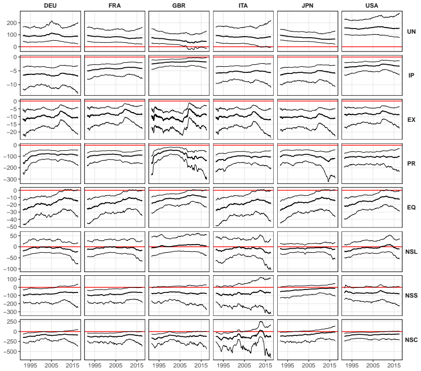
On its own terms, the central discovery is that the estimated log-volatility process $h_t$ behaves like a meaningful international uncertainty measure: it rises around the Asian and Russian crises, 9/11, the Iraq War, the global financial crisis, the European sovereign debt crisis, and the Brexit/Trump period, and it tracks established proxies such as GPR, GEPU, WUI and the VIX. Treating an innovation to $h_t$ as an exogenous uncertainty shock, the model finds significant increases in unemployment (up to eight basis points in the United States), declines in industrial production, exports, inflation and equity prices, and a flattening of the yield curve across all six countries. The responses are not constant: cumulative effects on equity prices and some other variables diminish over the sample, and the strength of the real effects varies over time, with muted effects in the aftermath of the Great Recession for several series.
Load-bearing premise
The whole approach depends on treating the single estimated volatility component as an exogenous uncertainty shock that arrives before the economy moves, rather than as a symptom of movements already under way.
Editorial extensions
If this is right
- The estimated $h_t$ series can serve as an international uncertainty indicator that peaks at the global financial crisis, the European sovereign debt crisis, and the Brexit/Trump episodes, and moves with GPR, GEPU, WUI and VIX.
- Uncertainty shocks raise unemployment in every country in the sample, with the largest cumulative effects in Germany and the United States.
- Industrial production, exports, inflation and equity prices fall in response to an uncertainty shock, and the yield curve flattens as term spreads narrow.
- The strength of these effects changes over time: equity-price responses shrink across the sample, and post-Great-Recession responses are muted for several real variables before reverting later.
Reading between the lines
- Editorial extension: the identification of $h_t$ could be stress-tested by re-estimating the model with zero restrictions that keep slow-moving real variables from responding on impact; if the impulse responses change materially, the uncertainty-first ordering is doing the work.
- Editorial extension: because $h_t$ is extracted from six advanced economies, applying the same machinery to a panel that includes emerging markets could reveal whether the scalar factor remains international or becomes a proxy for US or European stress.
- Editorial extension: the estimated $h_t$ could be exported as an observable regressor in single-country studies of uncertainty transmission, giving an external check on whether it captures information beyond text-based uncertainty indices.
Signed reviews
Editorial analysis
A structured set of objections, weighed in public.
Referee Report
Summary. The paper proposes a Bayesian global vector autoregression with drifting coefficients and factor stochastic volatility in mean for six advanced economies, using monthly data from 1991:04 to 2018:07. A scalar latent process h_t drives the common volatility of factor innovations and also enters the mean equations with country- and variable-specific coefficients. Estimation uses hierarchical normal-gamma priors that shrink the model toward constant coefficients and homoscedastic errors. The paper reports the estimated h_t as an international uncertainty measure, compares it with several text-based and VIX-based proxies, and presents impulse response functions to an uncertainty shock for unemployment, industrial production, exports, inflation, equity prices, and Nelson-Siegel yield-curve factors. The main empirical claim is that uncertainty shocks produce pronounced real and financial effects in all countries, with magnitudes and timing that differ across economies and over time.
Significance. If the results hold, the paper makes a useful methodological contribution by combining a global VAR with drifting parameters, factor stochastic volatility in mean, and hierarchical shrinkage priors, and it extends the international uncertainty literature to a joint treatment of time variation and cross-country heterogeneity. The appendices provide a fairly detailed MCMC algorithm, posterior credible intervals are reported, and the estimated uncertainty measure is compared with established proxies. The central quantitative claim, however, rests on an impulse-response object that is never formally defined in the manuscript. Because the reported magnitudes in Figures 4 and 5 and the abstract's 'pronounced real and financial effects' are read directly from that object, the significance is conditional on the authors supplying a precise definition of the uncertainty shock and its propagation, as well as a scale normalization for the latent h_t.
major comments (3)
- [Section 4.2, Eqs. (1)-(2), Appendix B] The impulse response to an international uncertainty shock is never defined. The paper does not state whether the shock is a one-unit change in the latent h_t, a one-standard-deviation innovation to the random walk h_t, or some other size; it does not specify how the shock is propagated through the mean equation (beta_it h_t) and the factor covariance exp(h_t)LL'; and it gives no baseline path or normalization of h_t. Footnote 7 states that detailed numerical tables are available only upon request, so Figures 4 and 5 cannot be reproduced from the manuscript as it stands. This is load-bearing because the abstract's quantitative conclusions are read directly from these figures, and footnote 1 reports that the likelihood is flat in sigma_h, so the response magnitudes are sensitive to the adopted normalization and shock definition.
- [Section 2.1, Eq. (1), Fig. 1] The scale and location of the latent process h_t are not identified from the likelihood: Var(epsilon_t) = exp(h_t)LL' + Omega_t is invariant to multiplying exp(h_t) by a constant and rescaling L and Omega_t accordingly, while the random walk for h_t has no location anchor. The paper fixes sigma_h = 0.2 but does not state a location normalization, such as a prior mean for h_0 or a sum-to-zero constraint. The posterior median values of h_t in the range of about -10 to -2 in Figure 1 are therefore arbitrary up to the prior. If the impulse response is a one-unit shock to h_t, the magnitudes in Section 4.2 depend directly on this normalization; if it is a sigma_h-standardized innovation, the magnitudes depend on the fixed value of sigma_h. The authors should state the normalization explicitly and show that the qualitative conclusions are robust to alternative normalizations.
- [Section 2.1, identification of the uncertainty shock] The recursive identification of an exogenous uncertainty shock is asserted rather than formalized. The text relates the approach to ordering uncertainty indices first, but h_t is an estimated latent process from the same system whose responses are then attributed to uncertainty shocks. Because the priors on beta_it are centered at zero and do not impose sign restrictions, the negative responses in Section 4.2 are data outcomes rather than imposed restrictions. As a correctness check, the authors should state explicitly what structural assumption identifies the innovation to h_t as an exogenous uncertainty shock, and report a robustness experiment, for example including lags of h_t in the mean or using an alternative ordering, that supports the causal interpretation.
minor comments (6)
- [Footnote 7] The statement that detailed tables are available upon request is not consistent with current reproducibility standards; please provide numerical impulse-response tables in the paper or in a supplementary file.
- [Section 4.1] There is a typo: "bancruptcy" should be "bankruptcy".
- [Appendix C] There is a typo: "simliar" should be "similar".
- [Figure 4 note] The note "1992:01 to 2017:07 on biannual frequency" does not explain how the color gradient maps to time; please clarify which colors represent early and late periods.
- [Section 4.2] Some statements about "significant" responses appear inconsistent with credible sets that cover zero, for example for industrial production and exports; please define the significance criterion used (e.g., 68% or 90% posterior interval excluding zero) and apply it consistently.
- [Section 3, Eq. (8)] The Nelson-Siegel decay parameter lambda is fixed at 0.0609 rather than estimated; since the yield-curve factors are constructed from this parameter, a brief sensitivity discussion would strengthen the results.
Circularity Check
No significant circularity: the uncertainty measure and the responses to uncertainty shocks are estimated from the model's own factor-SV structure, and the sign and magnitude of the responses are not imposed by the definition of h_t or by the priors.
full rationale
The paper's central claim is that a latent common factor volatility h_t, estimated jointly with a global VAR, is a valid measure of international uncertainty and that shocks to h_t have time-varying real and financial effects. This claim is not circular in the sense prohibited by the review rules. Equations (1) and (2) define h_t as the common log-volatility of latent factors, and h_t enters both the factor covariance and the mean of the process through the estimated coefficients beta_it. The impulse responses to an h_t shock are objects computed from the estimated posterior distribution of the model parameters and latent states; nothing in the definition of h_t, the factor stochastic volatility structure, or the hierarchical priors in Section 2.2 forces the responses to be negative for output or positive for unemployment. The priors center on a constant-parameter, homoscedastic specification and shrink coefficients toward common means, but they do not restrict the sign of beta_it or of the resulting impulse responses. The comparison with external uncertainty indices in Figure 2 is an ex-post validation exercise, not an input that determines the estimates. The only self-citation by the author, Fischer, Huber and Pfarrhofer (2019), is used as a comparison of prior constructions and is not load-bearing for the empirical identification. The paper does leave the impulse response definition underspecified: it does not state the shock size, normalization, or propagation algorithm for h_t, and footnote 7 says detailed tables are only available on request. This is a reproducibility and completeness concern, but it is not a circular reduction of the sort required for a circularity finding. The central derivation is self-contained: the latent uncertainty measure is identified from the factor-SV structure, and the response patterns are data-driven rather than imposed by construction.
Assumptions & free parameters
free parameters (4)
- sigma_h (innovation variance of uncertainty process ht) =
0.2
- Nelson-Siegel decay parameter lambda =
0.0609
- Prior hyperparameters d0 = d1 = 0.01 and a* ~ Exp(1) =
0.01 and 1
- Prior variance of constant impact coefficients beta_it =
10
assumptions (4)
- domain assumption The error terms follow a factor stochastic volatility structure with common scale exp(ht), so ht can be interpreted as the common international uncertainty factor.
- domain assumption ht and the idiosyncratic log-variances follow independent random walks, with fixed sigma_h = 0.2.
- domain assumption Innovations to ht can be ordered first and interpreted as exogenous international uncertainty shocks.
- standard math The MCMC algorithm in Appendices A and B correctly samples from the posterior.
invented entities (1)
-
ht, latent international uncertainty process
Cite this review
Pith. "Pith review of Measuring international uncertainty using global vector autoregressions with drifting parameters." pith.science (2026). https://pith.science/paper/NKAY3C5P
@misc{pith2026190806325,
  author       = {Pith},
  title        = {Pith review of: Measuring international uncertainty using global vector autoregressions with drifting parameters},
  year         = {2026},
  howpublished = {\url{https://pith.science/paper/NKAY3C5P}},
  note         = {Machine review of arXiv:1908.06325}
}
read the original abstract
This paper investigates the time-varying impacts of international macroeconomic uncertainty shocks. We use a global vector autoregressive specification with drifting coefficients and factor stochastic volatility in the errors to model six economies jointly. The measure of uncertainty is constructed endogenously by estimating a scalar driving the innovation variances of the latent factors, which is also included in the mean of the process. To achieve regularization, we use Bayesian techniques for estimation, and introduce a set of hierarchical global-local priors. The adopted priors center the model on a constant parameter specification with homoscedastic errors, but allow for time-variation if suggested by likelihood information. Moreover, we assume coefficients across economies to be similar, but provide sufficient flexibility via the hierarchical prior for country-specific idiosyncrasies. The results point towards pronounced real and financial effects of uncertainty shocks in all countries, with differences across economies and over time.
Figures


Figures from the paper (2 more)

Reference graph
Works this paper leans on
-
[1]
, " * write output.state after.block = add.period write newline
ENTRY address author booktitle chapter edition editor eid howpublished institution journal key month note number organization pages publisher school series title type volume year label extra.label sort.label short.list INTEGERS output.state before.all mid.sentence after.sentence after.block FUNCTION init.state.consts #0 'before.all := #1 'mid.sentence := ...
-
[2]
write newline
" write newline "" before.all 'output.state := FUNCTION n.dashify 't := "" t empty not t #1 #1 substring "-" = t #1 #2 substring "--" = not "--" * t #2 global.max substring 't := t #1 #1 substring "-" = "-" * t #2 global.max substring 't := while if t #1 #1 substring * t #2 global.max substring 't := if while FUNCTION word.in bbl.in " " * FUNCTION format....
-
[3]
Aastveit KA, Natvik GJJ, and Sola S (2013), Economic uncertainty and the effectiveness of monetary policy, Norges Bank Working Paper 17
work page 2013
-
[4]
Aguilar O, and West M (2000), Bayesian Dynamic Factor Models and Portfolio Allocation, Journal of Business and Economic Statistics 18(3), 338--357
work page 2000
-
[5]
Alessandri P, and Mumtaz H (2019), Financial regimes and uncertainty shocks, Journal of Monetary Economics 101, 31--46
work page 2019
-
[6]
Baker SR, Bloom N, and Davis SJ (2016), Measuring Economic Policy Uncertainty, Quarterly Journal of Economics 131(4), 1593--1636
work page 2016
-
[7]
Basu S, and Bundick B (2017), Uncertainty Shocks in a Model of Effective Demand, Econometrica 85(3), 937--958
work page 2017
-
[8]
Belmonte MA, Koop G, and Korobilis D (2014), Hierarchical Shrinkage in Time-Varying Parameter Models, Journal of Forecasting 33(1), 80--94
work page 2014
Show all 57 references
-
[9]
Berger T, Grabert S, and Kempa B (2016), Global and Country-Specific Output Growth Uncertainty and Macroeconomic Performance, Oxford Bulletin of Economics and Statistics 78(5), 694--716
2016
-
[10]
Bertolotti F, and Marcellino M (2019), Tax shocks with high and low uncertainty, Journal of Applied Econometrics forthcoming
2019
-
[11]
Bitto A, and Fr\"uhwirth-Schnatter S (2019), Achieving shrinkage in a time-varying parameter model framework, Journal of Econometrics 210(1), 75--97
2019
-
[12]
Bloom N (2009), The Impact of Uncertainty Shocks, Econometrica 77(3), 623--685
2009
-
[13]
Caballero RJ, Farhi E, and Gourinchas PO (2017), The Safe Assets Shortage Conundrum, Journal of Economic Perspectives 31(3), 29--46
2017
-
[14]
Caldara D, and Iacoviello M (2018), Measuring geopolitical risk, FRB International Finance Discussion Paper 1222
2018
-
[15]
Canova F, and Ciccarelli M (2004), Forecasting and turning point predictions in a Bayesian panel VAR model, Journal of Econometrics 120(2), 327--359
2004
-
[16]
--- --- --- (2013), Panel Vector Autoregressive Models: A Survey, ECB Working Paper Series 1507, 1--55
2013
-
[17]
Carriero A, Clark TE, and Marcellino M (2018 a ), Assessing international commonality in macroeconomic uncertainty and its effects, Federal Reserve Bank of Cleveland Working Paper 18-03
2018
-
[18]
--- --- --- (2018 b ), Measuring Uncertainty and Its Impact on the Economy, Review of Economics and Statistics 100(5), 799--815
2018
-
[19]
--- --- --- (2019), The Identifying Information in Vector Autoregressions with Time-Varying Volatilities: An Application to Endogenous Uncertainty, Federal Reserve Bank of Cleveland Working Paper 18-05
2019
-
[20]
Carriero A, Mumtaz H, Theodoridis K, and Theophilopoulou A (2015), The impact of uncertainty shocks under measurement error: A proxy SVAR approach, Journal of Money, Credit and Banking 47(6), 1223--1238
2015
-
[21]
Carter CK, and Kohn R (1994), On Gibbs sampling for state space models, Biometrika 81(3), 541--553
1994
-
[22]
Chan JC (2017), The stochastic volatility in mean model with time-varying parameters: An application to inflation modeling, Journal of Business & Economic Statistics 35(1), 17--28
2017
-
[23]
Crespo Cuaresma J, Doppelhofer G, Feldkircher M, and Huber F (2019), Spillovers from US monetary policy: Evidence from a time varying parameter global vector autoregressive model, Journal of the Royal Statistical Society: Series A (Statistics in Society) 182(3), 831--861
2019
-
[24]
Crespo Cuaresma J, Huber F, and Onorante L (2017), Fragility and the spillovers of international uncertainty shocks, WU Department of Economics Working Paper 245
2017
-
[25]
Diebold FX, and Li C (2006), Forecasting the term structure of government bond yields, Journal of Econometrics 130(2), 337--364
2006
-
[26]
Diebold FX, Rudebusch GD, and Aruoba SB (2006), The macroeconomy and the yield curve: a dynamic latent factor approach, Journal of Econometrics 131(1-2), 309--338
2006
-
[27]
Feldkircher M, and Huber F (2016), The international transmission of US shocks--Evidence from Bayesian global vector autoregressions, European Economic Review 81, 167--188
2016
-
[28]
Feldkircher M, Huber F, and Kastner G (2017), Sophisticated and small versus simple and sizeable: When does it pay off to introduce drifting coefficients in Bayesian VARs? ArXiv Preprint 1711.00564(v2)
2017 arXiv
-
[29]
Fern\' a ndez-Villaverde J, Guerr\' o n-Quintana P, Kuester K, and Rubio-Ram\' i rez J (2015), Fiscal Volatility Shocks and Economic Activity, American Economic Review 105(11), 3352--3384
2015
-
[30]
Fischer MM, Huber F, and Pfarrhofer M (2019), The regional transmission of uncertainty shocks on income inequality in the United States, Journal of Economic Behavior & Organization forthcoming
2019
-
[31]
Fr\" u hwirth-Schnatter S (1994), Data augmentation and dynamic linear models, Journal of Time Series Analysis 15(2), 183--202
1994
-
[32]
u hwirth-Schnatter S, T \
Fr \"u hwirth-Schnatter S, T \"u chler R, and Otter T (2004), Bayesian analysis of the heterogeneity model, Journal of Business & Economic Statistics 22(1), 2--15
2004
-
[33]
Fr\"uhwirth-Schnatter S, and Wagner H (2010), Stochastic model specification search for Gaussian and partial non-Gaussian state space models, Journal of Econometrics 154(1), 85--100
2010
-
[34]
Gilchrist S, Sim JW, and Zakraj s ek E (2014), Uncertainty, Financial Frictions, and Investment Dynamics, NBER Working Paper 20038
2014
-
[35]
Gilchrist S, Yankov V, and Zakraj s ek E (2009), Credit market shocks and economic fluctuations: Evidence from corporate bond and stock markets, Journal of Monetary Economics 56(4), 471--493
2009
-
[36]
Gilchrist S, and Zakraj s ek E (2012), Credit spreads and business cycle fluctuations, American Economic Review 102(4), 1692--1720
2012
-
[37]
Griffin JE, and Brown PJ (2010), Inference with normal-gamma prior distributions in regression problems, Bayesian Analysis 5(1), 171--188
2010
-
[38]
Huber F, and Feldkircher M (2019), Adaptive shrinkage in Bayesian vector autoregressive models, Journal of Business & Economic Statistics 37(1), 27--39
2019
-
[39]
Huber F, Koop G, and Onorante L (2019), Inducing Sparsity and Shrinkage in Time-Varying Parameter Models, Journal of Business & Economic Statistics forthcoming
2019
-
[40]
Jacquier E, Polson NG, and Rossi PE (2002), Bayesian Analysis of Stochastic Volatility Models, Journal of Business & Economic Statistics 20(1), 69--87
2002
-
[41]
Jurado K, Ludvigson SC, and Ng S (2015), Measuring uncertainty, American Economic Review 105(3), 1177--1216
2015
-
[42]
Kastner G (2019), Sparse Bayesian time-varying covariance estimation in many dimensions, Journal of Econometrics 210(1), 98--115
2019
-
[43]
Kastner G, and Fr\" u hwirth-Schnatter S (2014), Ancillarity-sufficiency interweaving strategy (ASIS) for boosting MCMC estimation of stochastic volatility models, Computational Statistics & Data Analysis 76, 408--423
2014
-
[44]
Koop G, and Korobilis D (2016), Model uncertainty in Panel Vector Autoregressive models, European Economic Review 81, 115--131
2016
-
[45]
Koopman SJ, and Hol Uspensky E (2002), The stochastic volatility in mean model: empirical evidence from international stock markets, Journal of Applied Econometrics 17(6), 667--689
2002
-
[46]
Ludvigson SC, Ma S, and Ng S (2019), Uncertainty and business cycles: exogenous impulse or endogenous response? American Economic Journal: Macroeconomics forthcoming
2019
-
[47]
u hwirth-Schnatter S, and Gr \
Malsiner-Walli G, Fr \"u hwirth-Schnatter S, and Gr \"u n B (2016), Model-based clustering based on sparse finite Gaussian mixtures, Statistics and Computing 26(1), 303--324
2016
-
[48]
Mumtaz H, and Musso A (2019), The Evolving Impact of Global, Region-Specific, and Country-Specific Uncertainty, Journal of Business & Economic Statistics 1--16
2019
-
[49]
Mumtaz H, and Surico P (2009), The Transmission of International Shocks: A Factor-Augmented VAR Approach, Journal of Money, Credit and Banking 41(S1), 71--100
2009
-
[50]
--- --- --- (2018), Policy uncertainty and aggregate fluctuations, Journal of Applied Econometrics 33(3), 319--331
2018
-
[51]
Mumtaz H, and Theodoridis K (2015), The international transmission of volatility shocks: An empirical analysis, Journal of the European Economic Association 13(3), 512--533
2015
-
[52]
--- --- --- (2017), Common and country specific economic uncertainty, Journal of International Economics 105, 205--216
2017
-
[53]
Journal of Business & Economic Statistics 36(2), 239--252
--- --- --- (2018), The Changing Transmission of Uncertainty Shocks in the U.S. Journal of Business & Economic Statistics 36(2), 239--252
2018
-
[54]
Mumtaz H, and Zanetti F (2013), The impact of the volatility of monetary policy shocks, Journal of Money, Credit and Banking 45(4), 535--558
2013
-
[55]
Nelson CR, and Siegel AF (1987), Parsimonious modeling of yield curves, Journal of Business 60(4), 473--489
1987
-
[56]
Pesaran MH, Schuermann T, and Weiner SM (2004), Modeling regional interdependencies using a global error-correcting macroeconometric model, Journal of Business and Economic Statistics 22(2), 129--162
2004
-
[57]
Verbeke G, and Lesaffre E (1996), A linear mixed-effects model with heterogeneity in the random-effects population, Journal of the American Statistical Association 91(433), 217--221
1996
Reviewed August 14, 2026 · model on record in the stance chip above.
Discussion (0). Continue with ORCID to comment.