REVIEW 3 major objections 6 minor 24 references
Fast Bayesian inference of Block Nearest Neighbor Gaussian process for large data
T0 review · 3 major / 6 minor · reviewed 2026-08-14 · deepseek-v4-flash
Pith's one-line read The block-NNGP is a valid spatial Gaussian process whose sparse block precision matrix makes Bayesian inference feasible for roughly $10^4$ locations, and it approximates the true process better than the NNGP when the spatial range is…
desk verdict Worth refereeing, but the headline superiority over NNGP rests on an uncontrolled more-neighbors comparison. read the letter →
The pith
A machine-rendered reading of the paper's core claim, the machinery that carries it, and where it could break.
The reading
What carries the argument
The central object is the block-conditional product in Eq. (2), defined on a chain graph whose nodes are locations, with directed edges from each location to its earlier neighbor blocks and undirected edges within each block. The chain-graph condition (with a directed acyclic subgraph picking one node per block) guarantees that the product is a proper joint density, and in the Gaussian case the resulting precision matrix is $\tilde{Q}_S = B_S^T F_S^{-1} B_S$, where $B_S$ contains the regression coefficients of each block on its neighbor blocks and $F_S$ is the block-diagonal conditional covariance matrix. This identity is the mechanism that converts local block-level regressions into a global sparse precision matrix, and the nonzero pattern of $\tilde{Q}_S$ is exactly the chain graph. INLA and sparse Cholesky routines then operate on this matrix, storing only $M$ small dense matrices rather than an $n\times n$ covariance.
What would settle it
A concrete test: simulate a spatial Gaussian process with smooth Matérn covariance ($\nu=1.5$) and effective range equal to half the domain diameter, fit block-NNGP with $M=64$ blocks and $n_b=2$ neighbor blocks alongside NNGP with $n_b=5$ neighbors, and check whether the block-NNGP posterior for the decay parameter is less biased and its predictive score better; if the NNGP wins, the claimed advantage at large ranges fails.
Extended reading notes
Core claim
The paper's central claim is that replacing the exact sequential factorization of a Gaussian process, Eq. (1), with the block-conditional product $\tilde{\pi}(w_S)=\pi(w_{b_1})\prod_{k=2}^M \pi(w_{b_k}|w_{N(b_k)})$ does not destroy the process: under a chain-graph condition the product is a genuine joint density, and for a Gaussian field it is the density of a Gaussian process with positive definite precision matrix $\tilde{Q}_S = B_S^T F_S^{-1} B_S$ that is sparse when each block has few neighbor blocks. Because the precision matrix is block-sparse, the block-NNGP can be embedded directly in INLA, giving fast approximate Bayesian inference at scale. Simulations and two real datasets (11,000 mining locations in Norway and 6,000 precipitation stations across South America) support the claim that the block-NNGP with only 2 to 6 neighbor blocks reproduces the empirical correlation better than the NNGP with 10 to 50 neighbors when the effective range is large or the field is smooth. The NNGP and independent spatial blocking are special cases, obtained with $M=n$ blocks or $n_b=0$ neighbors, respectively.
Load-bearing premise
The method stands on the assumption that conditioning each block on a small set of earlier neighbor blocks captures essentially all of the spatial dependence that matters, and the paper offers empirical support rather than a proven error bound for that assumption.
Editorial extensions
If this is right
- With the block-NNGP prior, Bayesian inference for large spatial datasets ($n\approx 10^4$) becomes a routine INLA computation, and the same machinery extends to non-Gaussian response models because the latent field remains a Gaussian Markov random field.
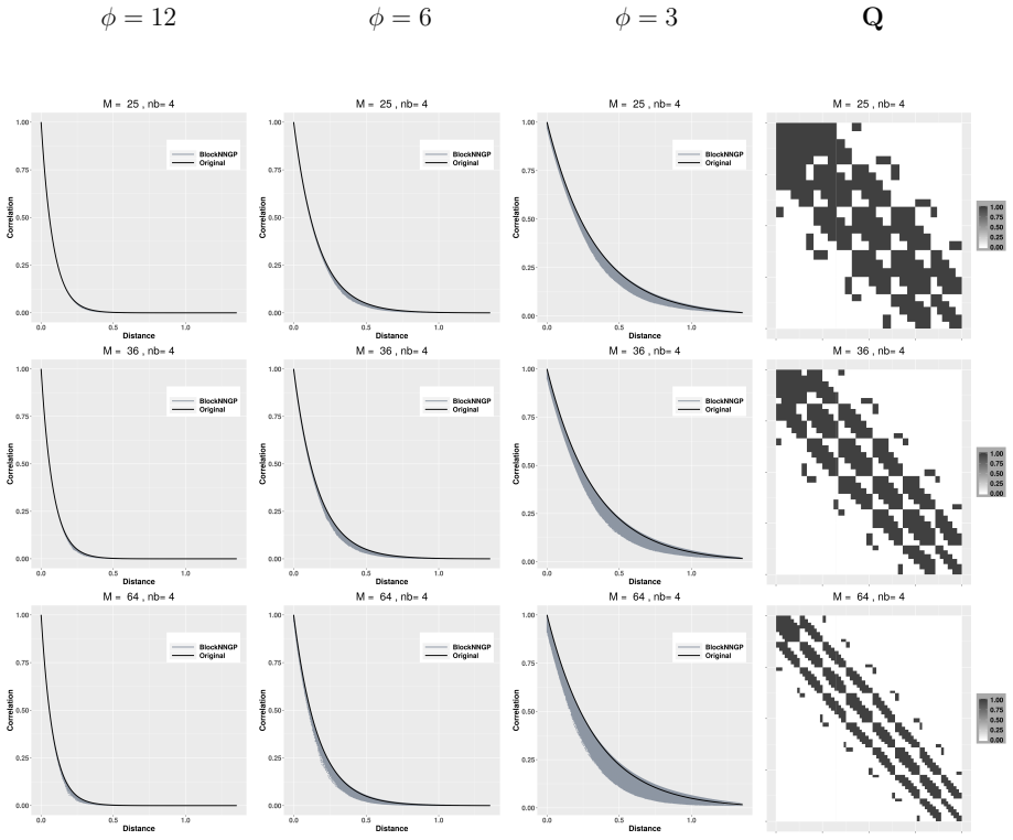
- For processes with large effective range or smooth Matérn covariance, block-NNGP with 2 to 6 neighbor blocks matches the true correlation and recovers parameters better than NNGP with 10 to 50 neighbors, so fewer neighbor parameters are needed for the same fidelity.
- The block-sparse precision matrix means the method stores only $M$ block matrices, inherits Cholesky bandwidth from the sparsity pattern, and is naturally parallel, so computation time drops as the number of blocks $M$ increases.
- Spatial prediction at new locations is cheap because each predictive location depends only on its own block's observed locations, and posterior predictive sampling is straightforward after inference.
- The framework unifies existing approaches: the NNGP is the $M=n$ special case and independent spatial blocking is the $n_b=0$ special case.
Reading between the lines
- A sharp theoretical bound on the Kullback-Leibler divergence between block-NNGP and the exact Gaussian process, as a function of block count, neighbor count, effective range, and smoothness, would turn the empirical advantage into a design rule for choosing $M$ and $n_b$; the paper leaves that bound open.
- Because the advantage is largest when dependence is smooth and long-ranged, block-NNGP is a natural candidate for spatio-temporal and multivariate extensions where global dependence is strong, directions the authors name as future work.
- The same block-conditional structure could be combined with local covariance tapering or SPDE-style approximations inside blocks to control small-scale and large-scale dependence separately; that combination is untested.
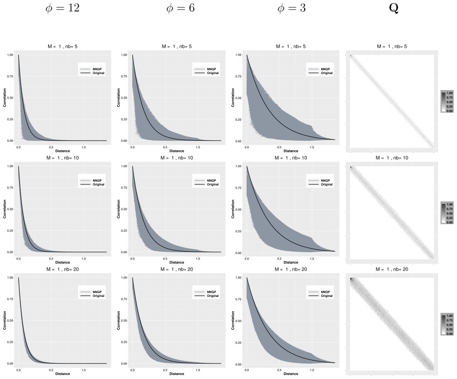
- A practical diagnostic suggested by the paper's figures is to compare the fitted process's empirical correlation with the theoretical covariance, since the match degrades under large $M$ or small $n_b$ and visually signals when more neighbor blocks are needed.
Signed reviews
Editorial analysis
A structured set of objections, weighed in public.
Referee Report
Summary. This paper proposes a block nearest-neighbor Gaussian process (block-NNGP) for large spatial datasets. The spatial domain is partitioned into blocks, and each block is modeled conditionally on a small number of earlier neighbor blocks, yielding a sparse block-structured precision matrix while retaining within-block dependence. The resulting Gaussian Markov random field is embedded as a prior in latent Gaussian models, and Bayesian inference is carried out with INLA, with a collapsed-MCMC alternative also described. The authors provide theoretical support via chain-graph arguments (Propositions 1 and 2, Lemma 1, Theorem 1), report simulations under different ranges and smoothness levels, and apply the model to mining and precipitation data with about 10^4 locations. The central practical claim is that block-NNGP approximates the original Gaussian process better than NNGP for large-range or smooth processes.
Significance. If the comparative claim were firmly established, the paper would be a useful addition to the large-spatial-data toolkit: block-NNGP naturally generalizes both NNGP and independent-block composite likelihoods, has a block-sparse precision matrix that is convenient for INLA, and extends to non-Gaussian responses through the latent-Gaussian-model framework. The theoretical construction is plausible and subsumes existing models as special cases. However, the current evidence does not convincingly support the headline claim of superiority over NNGP, because the comparisons are not cost-matched, and the formal statement of Proposition 1 contains an edge-direction error. These issues are fixable, but they are load-bearing for the paper's main message.
major comments (3)
- [Section 2, after Figure 4; Tables 2, 3, S1] The central claim that block-NNGP approximates the true GP better than NNGP for large-range or smooth processes is supported only by comparisons in which block-NNGP uses far more conditioning locations. The sentence 'since the block-NNGP is expected to have more neighbors than NNGP it will, necessarily, provide a better approximation to the full process' is not a proof, and the cited works (Guinness 2018; Banerjee 2020) do not establish this for the proposed blocking scheme. In the simulations, for example, block-NNGP with M=32 and nb=4 conditions each location on approximately 5*(2000/32)-1 ≈ 309 neighbors, whereas the NNGP models use 10 or 20 neighbors; similarly, in the precipitation application, block-NNGP with M=64 and nb=4 uses roughly 470 neighbors while the best NNGP uses 100. The real-data results are also mixed: in Table 3, NNGP(20) has RMSP 1.096 versus 1.176-1.223 for the block-NNGP models, and in Table S1, NNGP(100) is comparable to or better than the best block-NNGP. The evidence as presented supports 'more conditioning helps' rather than a structural advantage of block-NNGP. I request a controlled comparison at matched conditioning-set size, matched precision-matrix fill-in, or matched runtime, before asserting superiority.
- [Section 2, Proposition 1; Supplement A] The directed edge definition in Proposition 1 is reversed relative to the conditioning in Eq. (2). If the model uses π(w_bk | w_N(bk)), the standard directed-graph convention would place edges N(bk) → s_bk, not s_bk → N(bk). The proof in Supplement A is also very condensed: it invokes 'the last node from a DAG G_b' without specifying the topological order or proving that a block Δ(b1) can always be chosen so that no other term in Eq. (2) contains its nodes. Because Proposition 1 is the formal basis for the claim that ~π(w_S) is a joint density, this statement and its proof need to be corrected and rewritten with the correct edge orientation and a clear ordering argument.
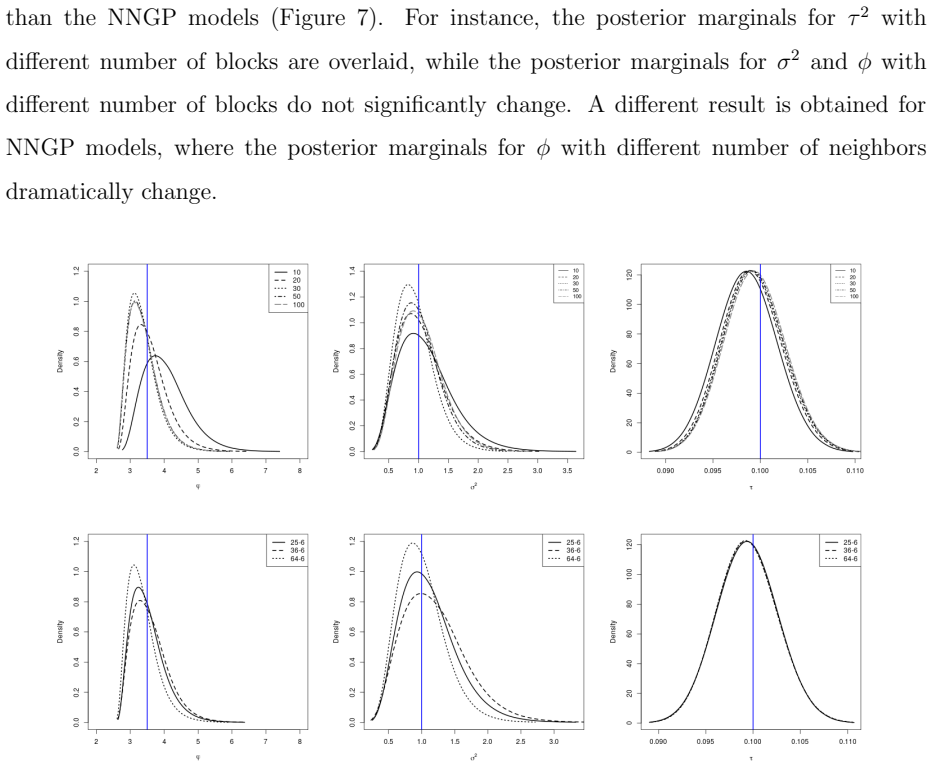
- [Section 3 and Section 4 applications] The empirical comparisons do not isolate the effect of the block structure from the effect of the number of neighbors. For instance, the statement in Section 3 that 'the NNGP model needs ≥ 30 neighbors to achieve a similar goodness of fit than the block-NNGP models with nb=4 and nb=6' does not account for the much larger conditioning sets used by block-NNGP. A fairer experiment would fix the total number of neighbors per location (or the number of nonzeros in the precision matrix) and compare NNGP and block-NNGP at that cost. Without such a comparison, the paper's title claim and the conclusion that 'block-NNGP performs better than the NNGP when the range is large or the spatial process is smoother' are not yet established.
minor comments (6)
- [Table 1] The credible intervals for φ and τ² appear to be swapped in the (I) M=128 column: the φ row shows (0.08, 0.12) and the τ² row shows (8.49, 14.5).
- [Figure 4 caption and text] The lower panel is described as the square-root KLD 'as a function of the number of observations' but the text says 'different number of neighbors'; the axis label should read 'number of neighbors'.
- [Eq. (4) and Lemma 1] The notation 's_i ⊂ b_k' should be 's_i ∈ b_k' in the definition of N(u_i) and in Lemma 1.
- [Supplement C] The sentence 'the computing times requirements for the block-NNGP models decreases as the number of neighbor blocks increases' appears to be reversed; the main text correctly states that time decreases as nb decreases.
- [Table 3 and text] The heading 'WAIC2' appears to be a typo for WAIC, and the text alternates between 'RSME' and 'RMSE' for the same quantity.
- [Supplement A, Proof of Proposition 2] The proof refers to '(iii) is proved' and '(ii) is proved' without an associated numbered list; the items being proved should be labeled explicitly.
Circularity Check
No significant circularity: the block-NNGP is built from an explicit conditional approximation of the GP, and its validation uses external simulations and held-out data; the uncontrolled neighbor-count comparison is an evidence concern, not a circular one.
full rationale
The derivation chain is self-contained: Eq. (2) starts from the exact factorization (1) and replaces each conditional π(w_bk | w_b1,...,w_b{k-1}) with π(w_bk | w_N(bk)); Proposition 1 and Proposition 2 (with proofs in Appendix A) show that the resulting product is a proper joint normal density with positive-definite block-sparse precision matrix ~Q_S = B_S^T F_S^{-1} B_S, and Lemma 1 and Theorem 1 verify the Kolmogorov conditions, so ~π defines a valid Gaussian process. None of these steps fits a parameter to the quantities being predicted. The KLD and SR-KLD comparisons in Figures 2-4 are computed directly from the true GP covariance and the approximate block-NNGP/NNGP covariances, and the simulation studies compare posterior summaries against known true values on held-out locations, so there is no fitted-input-called-prediction step. The main caveat is the sentence near Figure 4: 'since the block-NNGP is expected to have more neighbors than NNGP it will, necessarily, provide a better approximation to the full process. For a formal proof we refer to Guinness (2018); Banerjee (2020).' This is an appeal to external results and an uncontrolled comparison (block-NNGP conditions on many more points than the NNGP settings shown), but it is a question of evidence strength and experimental design, not a reduction of the central claim to its own definition. The paper's self-citations (Rue et al. 2009 for INLA, Lindgren et al. 2011 for SPDE background) are methodological, not load-bearing for the validity of block-NNGP. Overall, no circular step is exhibited.
Assumptions & free parameters
free parameters (2)
- number of blocks M =
varies: 8 to 450 in experiments
- number of neighbor blocks nb =
varies: 0 to 6 in most experiments
assumptions (4)
- domain assumption Each block w_bk is conditionally independent of all non-neighbor earlier blocks given its neighbor blocks w_N(bk) (Eq. 2).
- domain assumption The neighbor blocks N(bk) are chosen from the previous blocks in the fixed block ordering, so the block-level graph is acyclic.
- standard math Standard Gaussian conditional distribution formulas, Fubini's theorem, and matrix algebra results (positive definiteness, Schur complements) hold as background.
- domain assumption For prediction locations, each new location ui depends only on observed locations in the same block (N(ui) subset of the block's observed sites).
Cite this review
Pith. "Pith review of Fast Bayesian inference of Block Nearest Neighbor Gaussian process for large data." pith.science (2026). https://pith.science/paper/GZ6LEZXJ
@misc{pith2026190806437,
  author       = {Pith},
  title        = {Pith review of: Fast Bayesian inference of Block Nearest Neighbor Gaussian process for large data},
  year         = {2026},
  howpublished = {\url{https://pith.science/paper/GZ6LEZXJ}},
  note         = {Machine review of arXiv:1908.06437}
}
abstract
This paper presents the development of a spatial block-Nearest Neighbor Gaussian process (block-NNGP) for location-referenced large spatial data. The key idea behind this approach is to divide the spatial domain into several blocks which are dependent under some constraints. The cross-blocks capture the large-scale spatial dependence, while each block captures the small-scale spatial dependence. The resulting block-NNGP enjoys Markov properties reflected on its sparse precision matrix. It is embedded as a prior within the class of latent Gaussian models, thus Bayesian inference is obtained using the integrated nested Laplace approximation (INLA). The performance of the block-NNGP is illustrated on simulated examples and massive real data for locations in the order of $10^4$.
Figures

Figures from the paper (6 more)




Reference graph
Works this paper leans on
-
[1]
Abrahamsen, P. (1997). A review of gaussian random fields and correlation functions. Technical report
work page 1997
-
[2]
Banerjee, S. (2020). Modeling massive spatial datasets using a conjugate bayesian linear modeling framework. Spatial Statistics , 37:100417. Frontiers in Spatial and Spatio-temporal Research
work page 2020
-
[3]
Banerjee, S., Gelfand, A. E., Finley, A. O., and Sang, H. (2008). Gaussian predictive process models for large spatial datasets. Journal of the Royal Statistical Society, Series B , 70:825--848
work page 2008
-
[4]
Bentley, J. L. (1975). Multidimensional binary search trees used for associative searching. Commun. ACM , 18(9):509–517
work page 1975
-
[5]
Bolin, D. and Wallin, J. (2016). Spatially adaptive covariance tapering. Spatial Statistics , 18(Part A):163 -- 178
work page 2016
- [6]
-
[7]
Caragea, P. C. and Smith, R. L. (2007). Approximate likelihoods for spatial processes. In Joint Statistical Meetings - Section on Statistics & the Environment
work page 2007
-
[8]
Cressie, N. (1993). Statistics for Spatial Data . Wiley Classics Library
work page 1993
Show all 24 references
-
[9]
O., and Gelfand, A
Datta, A., Banerjee, S., Finley, A. O., and Gelfand, A. E. (2016). Hierarchical nearest-neighbor G aussian process models for large geostatistical datasets. Journal of the American Statistical Association , 111(514):800--812
2016
-
[10]
J., Tawn, J
Diggle, P. J., Tawn, J. A., and Moyeed, R. A. (1998). Model-based geostatistics. Journal of the Royal Statistical Society: Series C (Applied Statistics) , 47(3):299--350
1998
-
[11]
A., Reich, B
Eidsvik, J., Shaby, B. A., Reich, B. J., Wheeler, M., and Niemi, J. (2014). Estimation and prediction in spatial models with block composite likelihoods. Journal of Computational and Graphical Statistics , 23(2):295--315
2014
-
[12]
O., Datta, A., Cook, B
Finley, A. O., Datta, A., Cook, B. D., Morton, D. C., Andersen, H. E., and Banerjee, S. (2019). Efficient algorithms for bayesian nearest neighbor gaussian processes. Journal of Computational and Graphical Statistics , 28(2):401--414. PMID: 31543693
2019
-
[13]
Guinness, J. (2018). Permutation and grouping methods for sharpening gaussian process approximations. Technometrics , 60(4):415--429
2018
-
[14]
G., Schervish, M
Kaufman, C. G., Schervish, M. J., and Nychka, D. W. (2008). Covariance tapering for likelihood-based estimation in large spatial data sets. Journal of the American Statistical Association , 103(484):1545--1555
2008
-
[15]
Kaufman, C. G. and Shaby, B. A. (2013). The role of the range parameter for estimation and prediction in geostatistics. Biometrika , 100(2):473--484
2013
-
[16]
Lee, B. S. and Haran, M. (2019). Picar: An efficient extendable approach for fitting hierarchical spatial models. arXiv preprint arXiv:1912.02382
2019 arXiv
-
[17]
Lindgren, F., Rue, H., and Lindstr \"o m, J. (2011). An explicit link between G aussian fields and G aussian M arkov random fields: The SPDE approach. Journal of the Royal Statistical Society. Series B. Statistical Methodology , 73(4):423--498
2011
-
[18]
Liu, J. S. (1994). The collapsed gibbs sampler in bayesian computations with applications to a gene regulation problem. Journal of the American Statistical Association , 89(427):958--966
1994
-
[19]
Rue, H., Martino, S., and Chopin, N. (2009). Approximate bayesian inference for latent G aussian models by using integrated nested L aplace approximations. Journal of the Royal Statistical Society B , 71(2):319--392
2009
-
[20]
and Tjelmeland, H
Rue, H. and Tjelmeland, H. (2002). Fitting G aussian M arkov random fields to G aussian fields. Scandinavian Journal of Statistics , 29((1)):31--50
2002
-
[21]
Stein, M. L. (2013). Statistical properties of covariance tapers. Journal of Computational and Graphical Statistics , 22(4):866--885
2013
-
[22]
L., Chi, Z., and J.Welty, L
Stein, M. L., Chi, Z., and J.Welty, L. (2004). Approximating likelihoods for large spatial data sets. Journal of the Royal Statistical Society, Series B , 66(2):275--296
2004
-
[23]
Whittle, P. (1954). On stationary processes in the plane. Biometrika , 44:434--449
1954
-
[24]
write newline
" write newline "" before.all 'output.state := FUNCTION fin.entry add.period write newline FUNCTION new.block output.state before.all = 'skip after.block 'output.state := if FUNCTION new.sentence output.state after.block = 'skip output.state before.all = 'skip after.sentence '...
Reviewed August 14, 2026 · model on record in the stance chip above.
Discussion (0). Continue with ORCID to comment.