REVIEW 3 major objections 6 minor 33 references
Large-eddy simulation and modeling of Taylor-Couette flow with an outer stationary cylinder
T0 review · 3 major / 6 minor · reviewed 2026-08-14 · deepseek-v4-flash
Pith's one-line read This paper claims that in turbulent Taylor-Couette flow with a stationary outer cylinder, the torque ratio grows as the square root of the Taylor number divided by the square of a Lambert-W function, a logarithmic-corrected non-power law.
desk verdict A genuinely new analytic torque law for TC flow, but the central asymptotic claim hangs on a single fitted closure constant; worth refereeing. read the letter →
The pith
A machine-rendered reading of the paper's core claim, the machinery that carries it, and where it could break.
The reading
What carries the argument
The load-bearing construction is a one-dimensional, three-region radial model of the mean azimuthal velocity: region I is an inner-cylinder log layer with profile $U_\theta=\Omega_i R_i-u_{\tau i}(\kappa^{-1}\ln((r-R_i)u_{\tau i}/\nu)+A)$, region II has constant angular momentum $U_\theta=\frac{1}{2}\Omega_i R_i^2/r$, and region III is an outer log layer. The model is closed by the scaling relation $\delta_i=K u_{\tau i}/\Omega_i$, written as $\delta_i/d=\alpha Re_{\tau i}\eta/(Re_i(1-\eta))$ with $\alpha=2K=0.5$; this turns velocity matching at the inner-layer edge into a single algebraic equation for $Re_{\tau i}$. Solving that equation in the large-$Re_i$ limit introduces the Lambert-W function, whose sub-logarithmic growth produces the log-corrected torque law.
What would settle it
Measure $\delta_i$ and $u_{\tau i}$ separately in DNS or experiment at a second radius ratio, say $\eta=0.5$, over a range of $Re_i$: if $\delta_i\Omega_i/u_{\tau i}$ deviates from approximately 0.5 by more than the uncertainty, the closure—and with it the Lambert-W torque law—is falsified. Alternatively, bin existing $Nu(\mathrm{Ta})$ data at fixed $\eta$ by decade and check that the local slope drifts downward toward $1/2$ as $1/(\ln\mathrm{Ta})^2$ rather than settling on a constant exponent.
Extended reading notes
Core claim
The paper's claim is that the mean state of high-Reynolds-number Taylor-Couette flow with the outer cylinder at rest is captured quantitatively by matching two log-law layers against a known constant-angular-momentum core, $r u_\theta = \frac{1}{2}\Omega_i R_i^2$. The matching produces an algebraic equation for the inner friction Reynolds number $Re_{\tau i}$, and in the large-$Re_i$ limit the solution is $Re_{\tau i}\propto Re_i/W(Z_1)$ with $Z_1\propto \eta^{1/2}Re_i^{1/2}/(1-\eta)^{1/2}$. Converting to torque gives $Nu(\mathrm{Ta},\eta)=\kappa^2\eta^3\mathrm{Ta}^{1/2}/(4(1+\eta)^2 W(Z_2)^2)$ with $Z_2\propto \eta^{3/2}\mathrm{Ta}^{1/4}/((1-\eta)^{1/2}(1+\eta)^{3/2})$. At enormous $\mathrm{Ta}$ this becomes $Nu\sim 4\kappa^2\eta^3\mathrm{Ta}^{1/2}/((1+\eta)^2(\ln\mathrm{Ta})^2)$, a genuine non-power-law asymptote. The same model, extended with a Colebrook roughness function, predicts that a rough inner wall produces a fully rough plateau with $C_f$ independent of $Re_i$ and $Nu\sim\mathrm{Ta}^{1/2}$.
Load-bearing premise
The quantitative torque law rests on the assumption that the inner wall-layer thickness is proportional to the local friction velocity divided by the cylinder rotation speed, with the constant fixed at 0.5 from one DNS point; if that ratio depends on radius ratio or Reynolds number, the claimed asymptote fails.
Editorial extensions
If this is right
- At fixed $\eta<1$, $Nu(\mathrm{Ta})$ has no power-law asymptote; the true large-$\mathrm{Ta}$ behavior is $Nu\sim \mathrm{Ta}^{1/2}/(\ln\mathrm{Ta})^2$, so local power-law fits with exponent below $0.5$ must drift downward as $\mathrm{Ta}$ increases.
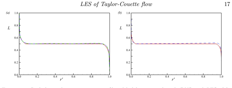
- The mean azimuthal flow approaches $u_\theta=\frac{1}{2}\Omega_i R_i^2/r$ across almost the whole gap, while the wall-layer thicknesses $\delta_i/d$ and $\delta_o/d$ shrink like the inverse of a Lambert-W function.
- The model reproduces DNS, LES, and experimental $Nu(\mathrm{Ta},\eta)$ data for $\eta=0.5$, $0.72$, and $0.909$ across $\mathrm{Ta}\simeq10^{10}$ to $10^{13}$, including the decline of inner-wall boundary-layer measures with $Re_i$.
- For a sand-grain-rough inner wall, the model predicts a fully rough plateau: $C_f$ independent of $Re_i$, $\delta_i/d$ independent of $Re_i$, and $Nu\sim\mathrm{Ta}^{1/2}$.
- The model is intended for practical radius ratios roughly $0.6\le\eta<1$; it does not cover the plane-Couette limit $\eta\to1$, where the predicted $\delta_i/d$ would diverge.
Reading between the lines
- If the Lambert-W form is generic, then single-exponent fits to $Nu(\mathrm{Ta})$ are inherently temporary; the local slope should decrease logarithmically with $\mathrm{Ta}$, a drift that can be checked by decade-binning existing torque data.
- The same three-region construction could be carried over to other rotating wall-bounded flows with roll-driven angular-momentum mixing, but the closure constant $K$ would need independent measurement rather than being assumed universal.
- The rough-wall branch gives a concrete engineering target: torque measurements on roughened cylinders should plateau as $Re_i$ grows, a Moody-diagram-style saturation that existing Taylor-Couette facilities could test directly.
- The deeper physical bet is that the constant-angular-momentum bulk persists to arbitrarily large $\mathrm{Ta}$; if Taylor rolls or the bulk itself change character at extreme driving, the asymptotic state would differ even if the wall-layer closure held.
Signed reviews
Editorial analysis
A structured set of objections, weighed in public.
Referee Report
Summary. The paper presents wall-resolved large-eddy simulations (LES) of Taylor–Couette flow with a rotating inner cylinder and a stationary outer cylinder at radius ratio η = 0.909 and inner Reynolds numbers up to Rei = 3×10^6, using the stretched-vortex subgrid model. The LES are verified against DNS at Rei = 10^5 and 3×10^5 and are then used to characterize the mean azimuthal velocity, turbulence intensities, and angular-momentum profiles. The authors propose a one-dimensional, three-region empirical model: log-law wall layers on each cylinder separated by a central region of constant angular momentum L = Ωi Ri^2/2. The model is closed by the scaling hypothesis δi = K uτ_i/Ωi, with the constant fixed to K = 0.25 (α = 2K = 0.5) using one DNS point. The model yields an analytic Lambert-W formula for Nu(Ta,η), predicts that Nu grows as Ta^{1/2} divided by the square of a Lambert-W function, and describes an asymptotic state of nearly constant angular momentum with vanishingly thin wall layers. An extension to sand-grain roughness predicts a fully rough regime with Nu ∼ Ta^{1/2} and Cf independent of Rei.
Significance. If the central closure is accepted, the paper provides a simple, closed-form description of the torque scaling in turbulent Taylor–Couette flow with a stationary outer cylinder, including a concrete non-power-law asymptote that could organize existing experimental and numerical data. The new wall-resolved LES data at Rei up to 3×10^6 for η = 0.909 are a useful resource, and the rough-wall extension gives a testable Moody-diagram analogue for this geometry. The algebraic derivations are transparent and the final formulas are easy to use. The main caveat is that the quantitative predictions and the asymptotic state are contingent on the empirically calibrated closure (4.7), and the paper would be strengthened by a clear statement of that conditionality and by a sensitivity analysis of the fitted constant.
major comments (3)
- [4.1] The closure δi = K uτ_i/Ωi is the sole load-bearing assumption of the model, yet it is introduced without derivation, and the constant is fixed by matching a single DNS point (Rei = 10^5, Reτi = 1410). That same DNS point reappears in the validation (Table 2 and Fig. 7), so the agreement there is a consistency check rather than an independent confirmation. The comparisons at other η (experiments) and at higher Rei (present LES) do provide indirect support for K being independent of η and Ta over the tested range, but the asymptotic claims in §4.6 and the non-power-law form in Eq. (4.15) rely on (4.7) holding at arbitrarily large Ta, far beyond the validated range. Please add a sensitivity study with respect to α (e.g., how Nu(Ta,η) and the inferred asymptotic state vary for α = 0.25, 0.5, 0.75, 1.0), and either present direct evidence for the scaling δi ∝ uτ_i/Ωi from DNS/LES at several η and Rei or explicitly frame the asymptotic state and the Lambert-W law as model-based conjectures in the abstract and conclusions.
- [4.2] The approximate analytical solution leading to Eq. (4.15) is obtained after substituting α = 1/2 into Eq. (4.9) and then dropping subdominant terms, and the final formula contains no dependence on α. This may mislead readers into thinking the Lambert-W expression is parameter-free. In reality, for α ≠ 1/2 the argument of the Lambert function acquires a factor √α (through the 2αη term in the logarithmic argument), and the quantitative prediction changes. Please state explicitly that the functional form—the logarithmic correction to Ta^{1/2}—is insensitive to the calibrated value, but that the specific formula (4.15) and the numerical comparisons are tied to α = 0.5.
- [3.1] The LES validation of the model at high Rei rests on a computational domain of Δθ = π/10 and Ly = 2πd/3. As the authors themselves note in §3.4, Ostilla-Monico et al. (2015b) found that finite-domain effects on the near-wall log region and on turbulence statistics are non-negligible at moderate Reynolds numbers. Because the high-Rei LES (up to Rei = 3×10^6) are used to support the model’s Ta dependence, the paper should quantify or at least discuss the possible influence of this narrow domain on the mean azimuthal velocity and torque, or clearly state the resulting uncertainty in the high-Rei validation.
minor comments (6)
- [§2.1–2.2] The heading 'Numerical method' appears twice; the second occurrence should be renumbered or renamed to distinguish the curvilinear formulation.
- [§2.2] The citation 'Cheng et al. 2017, 2018, ?' contains a bare question mark; the reference list is incomplete and should be fixed.
- [§4.5, Eq. (4.19)] The definition of δ99 uses the inequality U(r) - U_target < 0.01, which is not sign-definite; it should likely be |U(r) - U_target|/U_target < 0.01.
- [throughout] The spelling of the author name 'Ostilla-Monico' is inconsistent (e.g., Ostilla-M´onico vs. Ostilla-Mnico) in the text and in the reference list.
- [§4.5] The sentence 'Once the parameters Reτi and ηi have been determined' should refer to Reτi and δi rather than ηi.
- [Abstract] The abstract contains the sentence 'With Ri,Ro the inner and outer radii respectively, the radius ratio is η = 0.909', which reads as if the paper only treats one radius ratio, whereas the model is applied for η = 0.5, 0.72, and 0.909. Please rephrase to avoid confusion.
Circularity Check
The model's closure constant α is calibrated to a single DNS point that is then reused as a validation entry; the Lambert-W and asymptotic claims otherwise follow from the stated closure, so the circularity is partial, not total.
-
fitted input called prediction
[§4.1, Eqs. (4.7)–(4.10); Table 2]
"In their DNS of TC flow with η = 0.909, Ostilla-Mónico et al. (2016) report Reτi = 1410 at Rei = 10^5. Solving (4.9) with these parameters and with α = 0.25, 0.5, 0.75, 1.0 gives Reτi = 1529, 1418, 1360, 1323 respectively. For all subsequent calculations with the present model, we will use α = 0.5 which gives satisfactory agreement with DNS for this case."
The free parameter α=2K in the closure δ_i = K u_τi/Ω_i is chosen so that the model reproduces the DNS value Reτi=1410 at Rei=10^5, η=0.909. Table 2 then lists that same DNS value (1410) alongside the model outputs (1418 from Eq. (4.10), 1426 from Eq. (4.12)) as an apparent validation, and the same point enters the Nu(Ta) comparison of Fig. 7. Consequently, the agreement at this anchor point is enforced by the calibration rather than predicted independently. The remaining rows, other radius ratios, and the Lambert-W asymptotic structure are not fixed by this one point, so the circularity is local and does not reduce the central claim.
full rationale
The core derivation is self-contained: Eqs. (4.1)–(4.6) define a three-region log-layer model; Eq. (4.7) is an explicitly stated closure, not a hidden one; substituting it produces Eq. (4.10), whose approximate solution (4.12) has Lambert-W form, and combining with Eq. (4.14) yields the Nu(Ta,η) law (4.15). This is a genuine derivation conditional on the closure, not a renaming of data. The only clear circular step is the reuse of the DNS anchor point used to set α=0.5: that point appears again in Table 2 and in the Nu validation, so that particular agreement is by construction. However, the asymptotic logarithmic correction in Eq. (4.17) is independent of α, and the model is compared with independent experiments and DNS/LES at other Rei and η. The uniform-angular-momentum bulk (4.20) is assumed in region II of the model, so that element of the abstract's asymptotic state is a premise; the derived content is the wall-layer thinning and turbulence-intensity decline. Thus the central claim has substantive independent content, and the overall circularity score is 4 rather than higher.
Assumptions & free parameters
free parameters (1)
- alpha (closure coefficient) =
0.5
assumptions (3)
- domain assumption The mean azimuthal velocity in each wall layer follows the classical log law with kappa = 0.4 and A = 4.5.
- domain assumption A central region of constant angular momentum L = 0.5 exists between the wall layers and persists for arbitrarily large Taylor number.
- domain assumption The wall layers are thin enough that matching the log-law profiles at r = Ri + delta_i and r = Ro - delta_o with the constant-angular-momentum profile is a valid approximation.
Cite this review
Pith. "Pith review of Large-eddy simulation and modeling of Taylor-Couette flow with an outer stationary cylinder." pith.science (2026). https://pith.science/paper/OITVKOUY
@misc{pith2026190806577,
  author       = {Pith},
  title        = {Pith review of: Large-eddy simulation and modeling of Taylor-Couette flow with an outer stationary cylinder},
  year         = {2026},
  howpublished = {\url{https://pith.science/paper/OITVKOUY}},
  note         = {Machine review of arXiv:1908.06577}
}
abstract
We present wall-resolved large-eddy simulations (LES) of the incompressible Navier-Stokes equations together with empirical modeling for {turbulent} Taylor-Couette {(TC)} flow where the inner cylinder is rotating with angular velocity $\Omega_i$ and the outer cylinder is stationary. A simple empirical model of the turbulent, TC flow is developed consisting of near-wall, log-like turbulent wall layers separated by an annulus of constant angular momentum. The model is closed by a proposed scaling relation concerning the thickness of the wall layer on the inner cylinder. Model results include the Nusselt number $Nu$ (torque required to maintain the flow) and various measures of the wall-layer thickness as a function of both the Taylor {number} $Ta$ and $\eta$. These agree reasonably with experimental measurements, direct numerical simulation (DNS) and the present LES over a range of both $Ta$ and $\eta$. In particular, the model shows that, at fixed $\eta<1$, $Nu$ grows like $Ta^{1/2}$ divided by the square of the Lambert, (or Product-Log) function of a variable proportional to $Ta^{1/4}$. This cannot be represented by a power law dependence on $Ta$. At the same time the wall-layer thicknesses reduce slowly in relation to the cylinder gap. This suggests an asymptotic, very large $Ta$ state consisting of constant angular momentum in the cylinder gap with $u_\theta = 0.5\,\Omega_i\,R_i^2/r$, where $r$ is the radius, with vanishingly thin turbulent wall layers at the cylinder surfaces. An extension of the model to rough-wall turbulent wall flow at the inner cylinder surface is described. This shows an asymptotic, fully rough-wall state where the torque is independent of $Re_i/Ta$, and where $Nu\sim Ta^{1/2}$.
Figures


Figures from the paper (9 more)




Reference graph
Works this paper leans on
-
[1]
, " * write output.state after.block = add.period write newline
ENTRY address author booktitle chapter edition editor howpublished institution journal key month note number organization pages publisher school series title type volume year label extra.label sort.label short.list INTEGERS output.state before.all mid.sentence after.sentence after.block FUNCTION init.state.consts #0 'before.all := #1 'mid.sentence := #2 '...
-
[2]
write newline
" write newline "" before.all 'output.state := FUNCTION n.dashify 't := "" t empty not t #1 #1 substring "-" = t #1 #2 substring "--" = not "--" * t #2 global.max substring 't := t #1 #1 substring "-" = "-" * t #2 global.max substring 't := while if t #1 #1 substring * t #2 global.max substring 't := if while FUNCTION word.in bbl.in capitalize " " * FUNCT...
-
[3]
Andereck, C David, Liu, SS & Swinney, Harry L 1986 Flow regimes in a circular couette system with independently rotating cylinders. J. Fluid Mech.\/ 164 , 155--183
work page 1986
-
[4]
Cheng, W., Pullin, I, D. & Samtaney, R. 2018 Large-eddy simulation of flow over a rotating cylinder: the lift crisis at Re_D=6 10^4 . J. Fluid Mech. \/ 855 , 371--407
work page 2018
-
[5]
Cheng, W., Pullin, D. I. & Samtaney, R. 2018 Large-eddy simulation of flow over a grooved cylinder up to transcritical R eynolds numbers. J. Fluid Mech.\/ 835 , 327--362
work page 2018
-
[6]
Cheng, W., Pullin, D. I., Samtaney, R., Zhang, W. & Gao, W. 2017 Large-eddy simulation of flow over a cylinder with R e_ D from 3.9 10^ 3 to 8.5 10^ 5 : a skin-friction perspective. J. Fluid Mech.\/ 820 , 121–158
work page 2017
-
[7]
Chung, D. & Pullin, D. I. 2009 Large-eddy simulation and wall modelling of turbulent channel flow. J. Fluid Mech.\/ 631 , 281--309
work page 2009
-
[8]
Advances in Computational mathematics\/ 5 (1), 329--359
Corless, Robert M, Gonnet, Gaston H, Hare, David EG, Jeffrey, David J & Knuth, Donald E 1996 On the lambertw function. Advances in Computational mathematics\/ 5 (1), 329--359
work page 1996
Show all 33 references
-
[9]
Gao, Wei, Zhang, Wei, Cheng, Wan & Samtaney, Ravi 2019 Wall-modelled large-eddy simulation of turbulent flow past airfoils . J. Fluid Mech. \/ 873 , 174--210
2019
-
[10]
Annual review of fluid mechanics\/ 48 , 53--80
Grossmann, Siegfried, Lohse, Detlef & Sun, Chao 2016 High-- R eynolds number T aylor- C ouette turbulence. Annual review of fluid mechanics\/ 48 , 53--80
2016
-
[11]
M., Grossmann, Siegfried, Sun, Chao & Lohse, Detlef 2012 Ultimate turbulent taylor-couette flow
Huisman, Sander G., van Gils, Dennis P. M., Grossmann, Siegfried, Sun, Chao & Lohse, Detlef 2012 Ultimate turbulent taylor-couette flow. Phys. Rev. Lett.\/ 108 , 024501
2012
-
[12]
Huisman, Sander G., Scharnowski, Sven, Cierpka, Christian, K\"ahler, Christian J., Lohse, Detlef & Sun, Chao 2013 Logarithmic boundary layers in strong T aylor- C ouette turbulence. Phys. Rev. Lett.\/ 110 , 264501
2013
-
[13]
Hultmark, M., Vallikivi, M., Bailey, S. C. C. & Smits, A. J. 2012 Turbulent pipe flow at extreme R eynolds numbers. Phys. Rev. Lett.\/ 108 ( 9 )
2012
-
[14]
B., Marusic, I
Hutchins, N., Nickels, T. B., Marusic, I. & Chong, M. S. 2009 Hot-wire spatial resolution issues in wall-bounded turbulence. J. Fluid Mech.\/ 635 , 103–136
2009
-
[15]
Annual Review of Fluid Mechanics\/ 36 (1), 173--196
Jim\' e nez, Javier 2004 Turbulent flows over rough walls. Annual Review of Fluid Mechanics\/ 36 (1), 173--196
2004
-
[16]
2015 Direct numerical simulation of turbulent channel flow up to Re_ approximate to 5200
Lee, Myoungkyu & Moser, Robert D. 2015 Direct numerical simulation of turbulent channel flow up to Re_ approximate to 5200 . J. Fluid Mech.\/ 774 , 395--415
2015
-
[17]
Lundgren, T. S. 1982 Strained spiral vortex model for turbulent fine structure. Phys. Fluids\/ 25 (12), 2193--2203
1982
-
[18]
Physical Review E\/ 87 (2), 023014
Merbold, Sebastian, Brauckmann, HJ & Egbers, Christoph 2013 Torque measurements and numerical determination in differentially rotating wide gap T aylor- C ouette flow. Physical Review E\/ 87 (2), 023014
2013
-
[19]
& Pullin, D
Misra, A. & Pullin, D. I. 1997 A vortex-based subgrid stress model for large-eddy simulation. Phys. Fluids\/ 9 , 2443--2454
1997
-
[20]
& Moin, P
Morinishi, Y., Lund, T.S., Vasilyev, O.V. & Moin, P. 1998 Fully conservative higher order finite difference schemes for incompressible flow. Journal of Computational Physics\/ 143 (1), 90--124
1998
-
[21]
Ostilla-M \'o nico, Rodolfo, Verzicco, Roberto, Grossmann, Siegfried & Lohse, Detlef 2016 The near-wall region of highly turbulent T aylor- C ouette flow. J. Fluid Mech.\/ 788 , 95–117
2016
-
[22]
Physics of Fluids\/ 27 (2), 025110
Ostilla-Mónico, Rodolfo, Verzicco, Roberto & Lohse, Detlef 2015 a\/ Effects of the computational domain size on direct numerical simulations of T aylor- C ouette turbulence with stationary outer cylinder. Physics of Fluids\/ 27 (2), 025110
2015
-
[23]
Physics of Fluids\/ 27 (2), 746--325
Ostilla-Mónico, Rodolfo, Verzicco, Roberto & Lohse, Detlef 2015 b\/ Effects of the computational domain size on direct numerical simulations of T aylor- C ouette turbulence with stationary outer cylinder. Physics of Fluids\/ 27 (2), 746--325
2015
-
[24]
Pirozzoli, Sergio, Bernardini, Matteo & Orlandi, Paolo 2014 Turbulence statistics in couette flow at high R eynolds number. J. Fluid Mech.\/ 758 , 327--343
2014
-
[25]
Journal of Computational Physics\/ 228 (11), 4218 -- 4231
Simens, Mark P., Jiménez, Javier, Hoyas, Sergio & Mizuno, Yoshinori 2009 A high-resolution code for turbulent boundary layers. Journal of Computational Physics\/ 228 (11), 4218 -- 4231
2009
-
[26]
T., Morrill-Winter, C., Hutchins, N., Schultz, M
Squire, D. T., Morrill-Winter, C., Hutchins, N., Schultz, M. P., Klewicki, J. C. & Marusic, I. 2016 Comparison of turbulent boundary layers over smooth and rough surfaces up to high R eynolds numbers. J. Fluid Mech.\/ 795 , 210–240
2016
-
[27]
Taylor , G. I. 1923 Stability of a viscous liquid contained between two rotating cylinders. Philosophical Transactions of the Royal Society of London Series A\/ 223 , 289--343
1923
-
[28]
Van Gils, Dennis PM, Huisman, Sander G, Bruggert, Gert-Wim, Sun, Chao & Lohse, Detlef 2011 Torque scaling in turbulent T aylor- C ouette flow with co- and counter rotating cylinders. Phys. Rev. Lett.\/ 106 (2), 024502
2011
-
[29]
Van Gils, Dennis PM, Huisman, Sander G, Grossmann, Siegfried, Sun, Chao & Lohse, Detlef 2012 Optimal T aylor- C ouette turbulence. J. Fluid Mech.\/ 706 , 118--149
2012
-
[30]
Voelkl , T., Pullin , D. I. & Chan , D. C. 2000 A physical-space version of the stretched-vortex subgrid-stress model for large-eddy simulation . Phys. Fluids\/ 12 , 1810--1825
2000
-
[31]
Physics of Fluids\/ 11 (12), 3637--3649
Wereley, Steven T & Lueptow, Richard M 1999 Velocity field for taylor--couette flow with an axial flow. Physics of Fluids\/ 11 (12), 3637--3649
1999
-
[32]
Zang, Y., Street, R. L. & Koseff, J. R. 1994 A non-staggered grid, fractional step method for time-dependent incompressible N avier- S tokes equations in curvilinear coordinates. J. Comput. Phys.\/ 114 , 18--33
1994
-
[33]
& Samtaney, R
Zhang, W., Cheng, W., Gao, W., Qamar, A. & Samtaney, R. 2015 Geometrical effects on the airfoil flow separation and transition. Comput. Fluids\/ 15 , 60--73
2015
Reviewed August 14, 2026 · model on record in the stance chip above.
Discussion (0). Continue with ORCID to comment.