REVIEW 3 major objections 6 minor 19 references
Improving multilevel regression and poststratification with structured priors
T0 review · 3 major / 6 minor · reviewed 2026-08-14 · deepseek-v4-flash
Pith's one-line read Structured priors reduce bias in multilevel regression and poststratification estimates.
desk verdict A useful, careful MRP paper that shows structured priors help when the structure is real; the abstract promises a bit more than the evidence covers. read the letter →
The pith
A machine-rendered reading of the paper's core claim, the machinery that carries it, and where it could break.
The reading
What carries the argument
The load-bearing mechanism is the Gaussian Markov random field (GMRF) prior placed on a batch of varying intercepts: a sparse precision matrix that expresses which categories are neighbors and lets the model borrow information between them while remaining a proper Bayesian prior. For ordered categorical covariates the paper uses a first-order autoregressive prior, with $\rho \in (-1,1)$ learned from the data and a Beta$(0.5,0.5)$ hyperprior on $(\rho+1)/2$, and a random walk prior as the $\rho=1$ limiting case with a sum-to-zero constraint for identifiability; these shrink each age category's intercept toward its immediate neighbor. For spatial units it uses the BYM2 prior, a scaled mixture of an intrinsic conditional autoregressive (ICAR) component and an independent component, with penalized-complexity priors on precision and mixing, which lets adjacent areas share information without enforcing full spatial smoothness. Because a GMRF is a discrete approximation to a Gaussian process, the priors inherit an interpretation as smoothness-inducing function priors while remaining computationally tractable in the hierarchical regression.
What would settle it
Simulate a population whose true age preference is a sharp step function, flat until age 55 and flat at a very different level after, and measure absolute bias of the random walk MRP versus the independent-prior MRP under the same sampling regimes; if the random walk prior shows larger absolute bias than the baseline on several age categories, the claim that structured priors reduce bias regardless of how representative the survey is would fail for non-smooth truth. A second check is to apply the BYM2 spatial prior in an area where the true spatial effect has a hard boundary between adjacent regions and compare bias against the IID prior.
Extended reading notes
Core claim
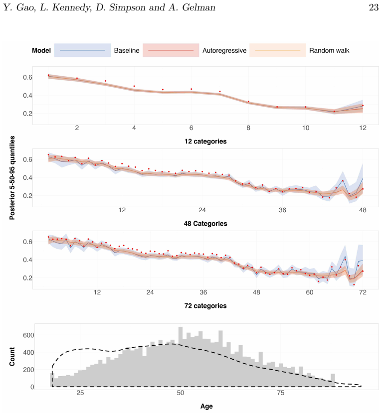
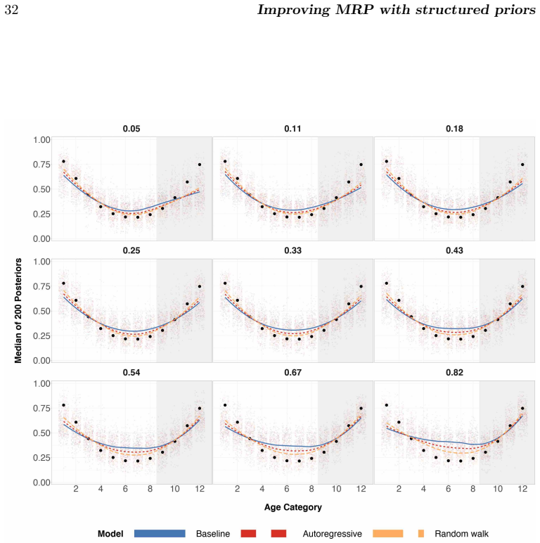
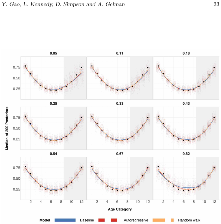
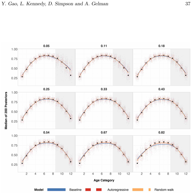
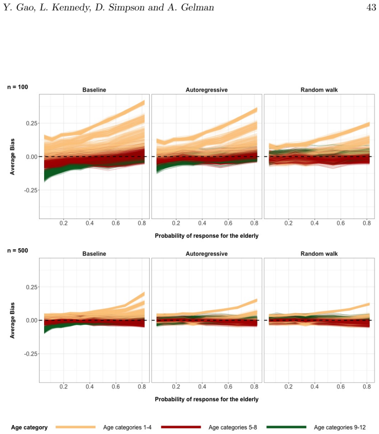
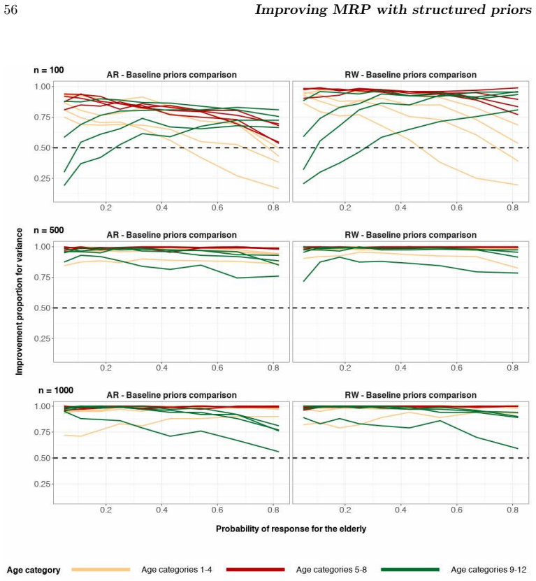
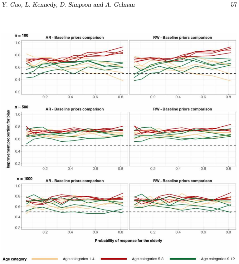
On the paper's own terms, the central discovery is that swapping the independent and identically distributed normal prior on a batch of varying intercepts for a Gaussian Markov random field prior, a first-order autoregressive or random walk prior for ordered categories such as age and a BYM2 spatial prior for geographic areas, reduces the absolute bias and the posterior standard deviation of posterior MRP estimates. Simulation evidence covers three age-preference shapes (U-shaped, cap-shaped, and increasing), sample sizes 100, 500, and 1000, and sampling probabilities for older adults perturbed from 0.05 to 0.82; the random walk prior consistently matches or beats the classical independent prior, with the largest gains, near ten percentage points in absolute bias, in the most extreme sampling regimes. A second simulation over the 52 PUMA areas of Massachusetts shows the BYM2 spatial prior beating an independent prior when the true spatial field is smooth, and behaving nearly identically when the truth is independent, indicating that the prior does not force structure that is absent. In the real-data analysis of support for same-sex marriage, the structured priors shrink posterior estimates for sparse age categories toward neighboring categories and stabilize posterior variances as the number of age categories grows from 12 to 72.
Load-bearing premise
The claim rests on the true population preference being smooth across the covariate that receives the structured prior, so the chosen smoothness assumption, similar ages behave similarly and adjacent areas behave similarly, matches reality; if the true effect jumps sharply between neighboring categories, the structured prior can over-smooth and increase bias, a situation the paper says it does not analyze.
Editorial extensions
If this is right
- Practitioners can adopt structured priors as a direct replacement for independent random effects on ordered or spatial covariates in MRP, keeping the same poststratification matrix and regression equation.
- MRP estimates made with these priors are less sensitive to who happens to be over- or under-represented in the sample, with the largest bias gains in extreme non-response regimes.
- With enough categories, around 12 or more, structured priors improve estimates; with very few categories the prior structure has little effect.
- When the true effect of a covariate is smooth, the random walk and BYM2 specifications also shrink posterior variance, giving tighter small-area intervals without trading away accuracy.
- Finer discretization of a continuous covariate is less costly under structured priors because neighboring categories stabilize each other, so analysts can model more age or income categories without variance blowing up.
Reading between the lines
- The same information-borrowing argument should extend to other ordered covariates in MRP, such as education levels, income brackets, or time periods, though the paper demonstrates it only for age and spatial adjacency.
- A natural next step, left open by the paper, is an adaptive smoothness prior that learns the degree of smoothing locally, which would soften the main risk of over-smoothing at genuine discontinuities in the covariate effect.
- Because GMRF priors approximate Gaussian process priors, the variance reduction seen here suggests that structured priors are a computationally cheap way to obtain part of GP-based regularization for survey estimates; the paper notes the link but does not pursue it empirically.
- One testable extension would be to apply the random walk prior to temporal MRP models used for tracking opinion over months or years, where neighboring time points should borrow strength in the same way neighboring age categories do.
Signed reviews
Editorial analysis
A structured set of objections, weighed in public.
Referee Report
Summary. The paper proposes replacing the independent normal varying intercepts in multilevel regression and poststratification (MRP) with Gaussian Markov random field priors for covariates with ordinal or spatial structure. Three specifications are compared: independent normal (baseline), first-order autoregressive, and random walk for age categories, plus BYM2 versus IID for spatial PUMAs. Evidence comes from simulation studies with three smooth age-preference curves and an ICAR-generated spatial truth across nine sampling-representativeness scenarios and sample sizes 100, 500, and 1000, followed by an application to the 2008 Annenberg phone survey with age discretized into 12, 48, and 72 categories. The paper claims that structured priors reduce absolute bias and posterior variance of MRP estimates in a large variety of data regimes.
Significance. The proposal is practically valuable if the claim is sustained: structured priors are a simple replacement for independent errors and can be implemented in standard software. Strengths include the public reproduction repository, the use of principled penalized complexity priors for hyperparameters, the BYM2 parameterization, and the real-data comparison across three discretizations. The main limitation is that the bias-reduction claim is demonstrated only for smoothly varying true effects; the paper's own conclusion acknowledges that the no-structure case is not analyzed, although an IID spatial robustness run is in fact reported. The central result is therefore best characterized as conditional on the prior class being compatible with the true covariate effect.
major comments (3)
- [4.1, 4.2, Abstract] The headline claim in the Abstract and the conclusion of Section 4.1 ("structured priors decrease absolute bias ... regardless of how representative the survey data are") is stronger than the simulation evidence supports. Every directed simulation uses a true age preference that is smooth (cap-shaped, U-shaped, or increasing; Section 4.1), and the spatial truth is drawn from an ICAR model (Section 4.2). The AR(1) and random walk priors in Eqs. (4.4) and (4.5) explicitly shrink neighboring age-category effects toward one another, so a step change or oscillatory true age effect could increase absolute bias near the discontinuity, particularly when one side of the discontinuity is under-sampled. The IID-truth spatial robustness check reported at the end of Section 4.2 is not a substitute: it tests the absence of structure, not a non-smooth but present structure. I ask the authors to add a simulation with a non-smooth true effect (for example, a step function or a rapidly alternating pattern) under the same nine sampling regimes, or to restrict the Abstract and Section 4.1 claims to the case where a smooth underlying pattern exists, as the conclusion already does.
- [6 vs 4.2] The Conclusion states that "we do not analyze the scenario when a structured prior is used for a covariate with no apparent structure," but Section 4.2 ends with exactly such an analysis: when XPUMA is generated from a multivariate independent normal, the BYM2 prior and the IID prior produce nearly the same posterior estimates. These two statements cannot both stand. Please either incorporate the IID-truth simulation into the main text as a formal robustness check with details, or delete the limitation sentence; as written, the manuscript both claims and disclaims this scenario, which makes it difficult to determine what evidence the authors intend to rely on.
- [5.3, 5.4, Abstract] The real-data analysis in Sections 5.3 and 5.4 confirms variance reduction and smoothing on the age covariate, but it cannot confirm bias reduction because no population truth is available. The wording in Section 5.4 correctly attributes variance reduction to the real-data application, whereas the Abstract's phrase "demonstrate their efficacy on non-representative US survey data" is potentially broader. I recommend adding a sentence in Section 5.4 that states explicitly that the real-data contribution is evidence about posterior variance and stability under discretization, not about bias reduction.
minor comments (6)
- [2] There is a duplicated word in the model specification: "for for k = 1,...,K" after the half-normal prior on sigma_k.
- [4.2] The word "probabillity" appears in the results section for the undirected structured priors and should be corrected to "probability."
- [4.1] The terms "probability of response," "probability vector of sampling," "completely random sample," and "fully representative" are used in ways that are easy to conflate; please define each precisely and distinguish equal response probabilities from sample proportions that match population cell sizes.
- [4.1] The claim that "absolute bias is reduced or stays the same for all age categories and all data regimes" is stronger than what can be verified from the plotted facets; please include a numeric table of mean absolute bias differences (structured minus baseline) by age category, sampling regime, and sample size.
- [Appendix B] The captions of Figures 37 and 38 report sampling probabilities of 0.81, 0.32, and 0.05, while the main text says the scenarios range from 0.05 to 0.82; these values should be harmonized.
- [4.2, Eq. (4.7)] The BYM2 scaling factor s is described qualitatively as computed so that the variance of the scaled ICAR component is approximately one; please provide the formula or a precise citation so that the implementation is fully reproducible.
Circularity Check
No significant circularity: the bias-reduction claims are empirical simulation results benchmarked against independently generated truths, not derivations equivalent to their inputs.
full rationale
The paper's central claim is that replacing iid varying intercepts with Gaussian Markov random field priors (AR(1), random walk, BYM2) reduces absolute bias and posterior variance in MRP. This claim is supported by simulation studies in which true cell preferences are generated from explicit smooth functions (U-shaped, cap-shaped, increasing) or from an ICAR field, and the fitted models are then compared against those true values. There is no step in which a parameter is fitted to the target quantity and then reported as a prediction: the posterior medians come from data simulated under the stated truth, and the truth is not used in fitting. The use of the authors' own PC priors and BYM2 parameterization is a borrowing of standard tools rather than a load-bearing self-citation; the paper writes out the model equations itself (e.g., Equations 4.4, 4.5, 4.7), and the simulation comparisons stand or fall on the data-generating processes and code, not on an imported uniqueness theorem. The fact that the simulated spatial truth is drawn from a GMRF, and the age truths are smooth, is an explicit modeling assumption that favors the structured priors; the paper also acknowledges in the conclusion that the mismatch scenario is not analyzed. That is a scope limitation or correctness risk, not circular reasoning. The IID-truth robustness check in Section 4.2 shows the authors test what happens when the structured prior is misspecified, and it does not force spatial structure when absent. Nothing in the derivation chain equates the predicted estimates to the inputs by construction, and the real-data analysis is an external application rather than a circular validation.
Assumptions & free parameters
free parameters (2)
- Simulation true outcome coefficients =
beta0 = 0 (increasing) or -1.5 (U/cap); betaState = 0.5; betaRelig = -0.5; effect vectors in appendix
- Number of age categories in simulations =
12 (with 48 and 72 in the application)
assumptions (3)
- domain assumption The true outcome is a smooth function of the structured covariate (age or space).
- domain assumption The poststratification matrix from the 5-year ACS represents the true target population.
- domain assumption Sampling with replacement approximates sampling without replacement from a very large population in the simulations.
Cite this review
Pith. "Pith review of Improving multilevel regression and poststratification with structured priors." pith.science (2026). https://pith.science/paper/MX53S423
@misc{pith2026190806716,
  author       = {Pith},
  title        = {Pith review of: Improving multilevel regression and poststratification with structured priors},
  year         = {2026},
  howpublished = {\url{https://pith.science/paper/MX53S423}},
  note         = {Machine review of arXiv:1908.06716}
}
read the original abstract
A central theme in the field of survey statistics is estimating population-level quantities through data coming from potentially non-representative samples of the population. Multilevel Regression and Poststratification (MRP), a model-based approach, is gaining traction against the traditional weighted approach for survey estimates. MRP estimates are susceptible to bias if there is an underlying structure that the methodology does not capture. This work aims to provide a new framework for specifying structured prior distributions that lead to bias reduction in MRP estimates. We use simulation studies to explore the benefit of these prior distributions and demonstrate their efficacy on non-representative US survey data. We show that structured prior distributions offer absolute bias reduction and variance reduction for posterior MRP estimates in a large variety of data regimes.
Figures


Figures from the paper (39 more)












Reference graph
Works this paper leans on
-
[1]
Bayesian hierarchical weighting adjustment and survey inference
Annenberg Center (2008). “The Annenberg Public Policy Center’s National Annen- berg Election Survey 2008 Phone Edition (NAES08-Phone) [Data file and code book].” Available from https://www.annenbergpublicpolicycenter.org/tag/ data-sets/. Besag, J. (1975). “Statistical analysis of non-lattice data.” Journal of the Royal Statis- tical Society: Series D (The ...
work page Pith review arXiv 2008
-
[3]
Sample size Age preference curve Poststrat
Table 4 below summarizes posterior quantile differences for the three true preference curves when the probability of sampling index is perturbed. Sample size Age preference curve Poststrat. cell bias Bias for each age category Improvement proportion 100 U-shaped Figure 3 Figure 7 Figure 30 500 U-shaped Figure 3 Figure 8 Figure 30 1000 U-shaped Figure 23 Fi...
work page 2010
-
[4]
Finally, XPUMA is a random sample coming an ICAR model {Ui}52 i=1 with a sum-to-zero constraint. Appendix B: Additional tables, definitions and figures for the data analysis The baseline, autoregressive and random walk specifications in the analysis of the 2008 Annenberg phone survey have in common the prior distributions defined in Equation 6.1. αEthnicity j...
work page 2008
-
[5]
2014/10/16 file: sample.tex date: May 26, 2020 Y
imsart-ba ver. 2014/10/16 file: sample.tex date: May 26, 2020 Y. Gao, L. Kennedy, D. Simpson and A. Gelman 31 Figure 6: Percentage proportions of data in every state for the Annenberg survey (top) and Annenberg percentage proportions - ACS percentage proportions (bottom). The proportions in both surveys were rounded to two decimal places. A state with gre...
work page 2014
-
[6]
The difference in proportions between Annenberg phone survey and the 2006-2010 5-year American Community Survey, broken down by state, is shown in the bottom heatmap of Figure
work page 2006
-
[8]
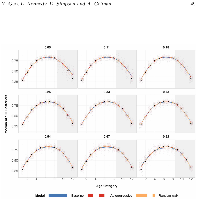
Black circles are true preference probabilities for each age group. The numerical index for the 9 plots correspond to the expected proportion of the sample that are older adults (also known as the probability of sampling the subpopulation group with age categories 9-12). The shaded gray region corresponds to the age categories of older individuals for whi...
work page 2014
-
[9]
Black circles are true preference probabilities for each age group. The numerical index for the 9 plots correspond to the expected proportion of the sample that are older adults (also known as the probability of sampling the subpopulation group with age categories 9–12). The shaded gray region corresponds to the age categories of older individuals for whi...
work page 2014
-
[10]
Black circles are true preference probabilities for each age group. The numerical index for the 9 plots correspond to the expected proportion of the sample that are older adults (also known as the probability of sampling the subpopulation group with age categories 9–12). The shaded gray region corresponds to the age categories of older individuals for whi...
work page 2014
Show all 19 references
-
[11]
Black circles are true preference probabilities for each age group. The numerical index for the 9 plots correspond to the expected proportion of the sample that are older adults (also known as the probability of sampling the subpopulation group with age categories 9–12). The s...
2014
-
[13]
y = 0 represents zero bias
The true preference curve for age is U-shaped. y = 0 represents zero bias. imsart-ba ver. 2014/10/16 file: sample.tex date: May 26, 2020 Y. Gao, L. Kennedy, D. Simpson and A. Gelman 49 Figure 24: Posterior medians for 100 simulations with 12 age groups, where true age preferen...
2014
-
[14]
Black circles are true preference probabilities for each age group. The numerical index for the 9 plots correspond to the expected proportion of the sample that are older adults (also known as the probability of sampling the subpopulation group with age categories 9–12). The s...
2014
-
[15]
y = 0 represents zero bias
The true preference curve for age is cap-shaped. y = 0 represents zero bias. imsart-ba ver. 2014/10/16 file: sample.tex date: May 26, 2020 52 Improving MRP with structured priors Figure 27: Posterior medians for 100 simulations with 12 age groups, where true age preference is ...
2014
-
[16]
Black circles are true prefer- ence probabilities for each age group. The numerical index for the 9 plots correspond to the expected proportion of the sample that are older adults (also known as the proba- bility of sampling the subpopulation group with age categories 9–12). T...
2014
-
[17]
y = 0 represents zero bias
The true preference curve for age is increasing-shaped. y = 0 represents zero bias. imsart-ba ver. 2014/10/16 file: sample.tex date: May 26, 2020 Y. Gao, L. Kennedy, D. Simpson and A. Gelman 55 Figure 30: The proportion of the time that structured priors have lower absolute po...
2014
-
[18]
The left column corresponds to the BYM2 spatial prior for PUMA effect
The possible values of average bias are in the interval (−1, 1). The left column corresponds to the BYM2 spatial prior for PUMA effect. The right column corresponds to an IID prior for PUMA effect. The probabilities 0.81, 0.32 and 0.05 in the top, middle and bottom rows respecti...
2014
-
[19]
The left column corresponds to the BYM2 spatial prior for PUMA effect
The possible values of average bias are in the interval (−1, 1). The left column corresponds to the BYM2 spatial prior for PUMA effect. The right column corresponds to an IID prior for PUMA effect. The probabilities 0.81, 0.32 and 0.05 in the top, middle and bottom rows respecti...
2014
-
[100]
Black circles are true preference prob- abilities for each age group. The numerical index for the 9 plots correspond to the expected proportion of the sample that are older adults (also known as the probability of sampling the subpopulation group with age categories 9-12). The...
2014
-
[500]
Black circles are true preference prob- abilities for each age group. The numerical index for the 9 plots correspond to the expected proportion of the sample that are older adults (also known as the probability of sampling the subpopulation group with age categories 9-12). The...
2014
-
[1000]
Black circles are true preference probabilities for each age group. The numerical index for the 9 plots correspond to the expected proportion of the sample that are older adults (also known as the probability of sampling the subpopulation group with age categories 9–12). The s...
2014
Reviewed August 14, 2026 · model on record in the stance chip above.
Discussion (0). Continue with ORCID to comment.