REVIEW 3 major objections 5 minor 34 references
Geographically-dependent individual-level models for infectious diseases transmission
T0 review · 3 major / 5 minor · reviewed 2026-08-14 · deepseek-v4-flash
Pith's one-line read A disease model that adds location to individual-level transmission recovers hidden spatial risk from outbreak data.
desk verdict A useful but incremental extension of ILMs with a real identification problem in the applied distance-decay conclusion. read the letter →
The pith
A machine-rendered reading of the paper's core claim, the machinery that carries it, and where it could break.
The reading
What carries the argument
The load-bearing object is the spatial random effect $\varphi_k$ inside the susceptibility function $\Omega_S(i,k)=\exp(\alpha + X(i,k)'\alpha_1 + X(k)'\alpha_2 + X(k,t-\rho)'\alpha_3 + \varphi_k)$, with $\boldsymbol{\varphi}$ following the LCAR prior $\boldsymbol{\varphi}\sim \text{MVN}(0, \sigma^2[\lambda R + (1-\lambda)I]^{-1})$, where $R$ encodes first-order neighbourhood structure. This prior does the work of letting nearby areas share unexplained risk while allowing independent noise, and the spatial dependence parameter $\lambda$ controls the balance. Transmission between areas is handled by the power-law kernel $d_{ij}^{-\delta}$, and the region-restricted variant restricts infectious contacts to the same area and its neighbours, which is what keeps the MCMC likelihood computable.
What would settle it
Simulate an epidemic with a strong distance-decay kernel (large $\delta$) and recorded infection times equal to true infection times plus an area-dependent diagnosis lag; fit the GD-ILM using the recorded times. If the posterior $\delta$ shrinks toward the Calgary value near $0.134$ and the $\varphi_k$ absorb the lag pattern, the flat-distance result in the real data could arise from event-time misspecification alone.
Extended reading notes
Core claim
The central claim is that a previously defined discrete-time ILM, in which the infection kernel depends only on separation, can be replaced by a geographically-dependent ILM whose susceptibility term includes an exponentiated area effect $e^{\varphi_k}$. With $\boldsymbol{\varphi}=(\varphi_1,\ldots,\varphi_K)$ assigned an LCAR prior, the model can separate observable covariates, unobserved spatially structured risk, and distance-based transmission in a single Bayesian MCMC fit. The paper's simulation evidence shows that credible intervals cover the true values when the fitted and generating models agree, and that spatial random effects remain close to truth under weak, moderate, and strong spatial dependence; fitting a region-restricted model to globally generated data biases only $\delta$ downward. Applied to 2009 Calgary influenza data, the fitted SIR model gives a population-size coefficient of about $0.714$ and a distance-decay parameter of about $0.134$, leading the authors to conclude that population size and local-area random effects, not centroid distance, dominate local transmission.
Load-bearing premise
The likelihood treats infection and removal times as known; the Calgary application sets infection time to the first physician-visit diagnosis date and fixes the infectious period, so if the delay between true infection and diagnosis varies across areas, the distance and spatial-effect estimates are biased.
Editorial extensions
If this is right
- In the Calgary SIR fit, the posterior mean population-size effect is $0.714$ with a 95% credible interval of roughly $0.619$ to $0.807$, so more populous dissemination areas contribute more to influenza pressure.
- The small posterior distance-decay estimate, $\delta \approx 0.134$, implies nearly flat infection-probability curves over distances of a few kilometres, which the paper interprets as distance between area centroids being a weak predictor of early spread.
- The posterior mean spatial effects separate clearly across the sixteen local geographic areas, so the model can rank areas by latent risk; the authors use these effects to construct posterior infectivity-rate risk maps for surveillance.
- Simulations show that the region-restricted fitting procedure recovers parameters when the model is correctly specified, and that mismatch from a global generating model shows up mainly as downward bias in $\delta$.
- Because the model is embedded in a Bayesian MCMC framework, the same machinery can be reused for other compartmental structures, such as SEIR or SIRS, without changing the core spatial-prior mechanism.
Reading between the lines
- If true infection times lag first physician-visit dates by an amount that varies across areas, the infectious pressure assigned to $\delta$ and $\varphi_k$ would be redistributed; re-running the Calgary analysis with data-augmented infection times could either confirm or erase the flat-distance conclusion.
- Because the units are dissemination areas rather than people, a fixed three-day infectious period at area level is a strong simplification; allowing within-area infection chains and variable infectious periods would test whether the distance effect remains small.
- The posterior infectivity-rate risk maps suggest a direct prospective test: rank local geographic areas by posterior mean daily infectivity early in an outbreak and compare that ranking with subsequent laboratory-confirmed or physician-visit counts.
- The same spatial-random-effect construction could be carried into epidemic forecasting models, where the posterior distribution of $\varphi_k$ would provide a data-driven prior for the next season's outbreak in the same set of areas.
Signed reviews
Editorial analysis
A structured set of objections, weighed in public.
Referee Report
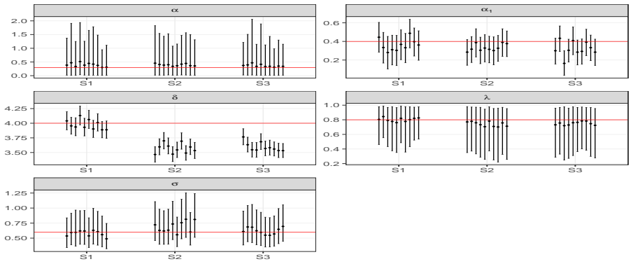
Summary. The paper extends the individual-level models (ILMs) of Deardon et al. (2010) to a new class of geographically-dependent ILMs (GD-ILMs) that incorporate area-level spatial random effects via an LCAR prior. This allows the model to separate observable covariates (e.g., DA population size), unobserved spatially structured risk at the LGA level, and distance-based transmission. The model is fitted with MCMC (Gibbs sampling and Metropolis-Hastings), and its performance is explored through simulations under three scenarios: a matched region-restricted model (S1), and two mismatch scenarios (S2, S3) where data are generated from a global transmission model but fitted with the region-restricted model, the latter showing systematic underestimation of the spatial kernel parameter δ. The method is then applied to the 2009 Calgary seasonal influenza outbreak at the dissemination-area level under SI and SIR frameworks, with the key applied finding that population size matters but spatial distance does not. The paper also presents posterior infectivity risk maps for the 16 Calgary LGAs.
Significance. If the claims hold, the GD-ILM framework is a useful methodological extension of ILMs, allowing area-level spatial heterogeneity to be modelled in a Bayesian fashion. The simulation study in S1 shows that parameters are recovered in the matched setting, which is an important positive result, and the MCMC implementation is described in sufficient detail to be reproducible. However, the applied conclusion that spatial distance is not an important factor is not supported by the presented analysis: the paper itself demonstrates that fitting the region-restricted model to global-transmission data produces underestimates of δ of the kind observed in the Calgary application. The significance of the methodological contribution is real, but the application requires substantial revision before the main applied claim can be accepted.
major comments (3)
- [Section 3.4 vs Section 4.3] The simulation study shows that when the data-generating model is global (Eq. 8) but the fitted model is region-restricted (Eq. 7), δ is consistently underestimated. The application in Section 4 fits exactly this region-restricted model to the Calgary data, with no evidence that transmission is confined to adjacent LGAs; the Discussion itself notes high human mobility across the city. The posterior δ ≈ 0.134 (SIR; CI 0.012, 0.288) is then interpreted in Section 4.3 as evidence that 'spatial distance was not an important factor.' This is precisely the pattern the paper's own simulations predict under a global-transmission mechanism, so the small δ does not discriminate between 'no distance effect' and 'region-restricted model misspecified.' The authors should fit the global model (Eq. 8) to the real data, or provide a formal model comparison or a credible justification for the region-restricted assumption, before drawing the applied conclusion about δ.
- [Section 2.3 and Section 4.2] The likelihood in Eq. (5) is derived under 'Assuming known infection and removal times.' In the application, the time a dissemination area becomes infectious is set to the first physician-visit diagnosis date, with a fixed infectious period of 3 days (SIR) or the whole study window (SI), an assumption the authors call 'naive' at the DA scale in Section 4.2. If true infection times differ from diagnosis dates by a lag that varies across areas, the infection pressure aggregates in Eq. (3) are misaligned and the estimates of δ, α1, and the φ_k may be biased. The Discussion explicitly defers event-time uncertainty to future work; the applied numerical results should be presented with this caveat prominently attached rather than as unqualified estimates.
- [Section 4.3, Figure 9] The infectivity risk maps in Figure 9 are posterior summaries of the fitted model's own spatial random effects, so the ranking of LGAs is in-sample and not validated against external outcomes. The statement that these maps 'may be used to inform targeted surveillance' is a suggestion, not an evaluated property; it should be framed as such, or supported by an out-of-sample prediction exercise.
minor comments (5)
- [Figure 6 caption] Panel (b) of Figure 6 is labeled 'κ(i,j) vs distance' but the text describes it as the posterior predictive distribution of infection probability against distance; this mismatch should be corrected.
- [Section 2.2.1 and Section 2.2.2] There are typos: 'in the the GD-ILMs' should be 'in the GD-ILMs', and 'matix' should be 'matrix'.
- [Section 4.3] The posterior estimates of λ are very close to 1 (0.982 and 0.986), the intrinsic CAR boundary at which the LCAR model is improper; the authors should discuss the potential for boundary effects and whether the uniform prior on λ in the application is appropriate given the near-boundary estimates.
- [Section 3.3] The prior specification for α, α1, and δ as 'positive half-normal priors, each with mode 0 and variance 100' is incomplete; specifying the scale parameter of the half-normal distribution explicitly would aid reproducibility.
- [Abstract and Section 4.3] The abstract mentions 'predicting future disease progression' but the paper does not perform forecasting or out-of-sample prediction; the risk maps are retrospective summaries. The framing should be tempered or a forecasting exercise added.
Circularity Check
No circular reduction found; low score reflects minor self-citation and in-sample risk-map summaries, not a fitted-input prediction.
full rationale
The paper's derivation chain is self-contained: the GD-ILM likelihood (Eqs. 3-6) is built explicitly from the infection probability and MCMC posterior, and the simulation study checks parameter recovery rather than re-labelling fitted values as predictions. The application's risk maps (Figure 9) are posterior summaries of the model's own α1 and φ_k parameters, and the paper does not validate them against external outcomes, so no fitted input is presented as an independent prediction. Citations to Deardon et al. (2010) provide the base ILM and computational background; since Deardon is an author this is a self-citation, but it is not load-bearing for the new CAR extension, and no uniqueness claim is imported from it. The acknowledged limitations (event-time uncertainty, Section 4.2; region-restricted fitting) are correctness/identifiability concerns, not circularity: the paper's own S2/S3 finding that δ is underestimated under model mismatch is a real threat to the Calgary 'distance not important' conclusion, but it does not make the derivation equivalent to its inputs. Score 2 reflects the minor self-citation and in-sample nature of the risk-map rankings, not a circular step.
Assumptions & free parameters
free parameters (7)
- α (constant infectivity rate) =
Set to 0 in the real-data analysis; 0.30 in simulations
- α1 (susceptibility covariate, DA population size) =
0.714 SIR (0.619, 0.807); 0.933 SI (0.837, 1.023)
- δ (power-law kernel decay) =
0.134 SIR (0.012, 0.288); 0.149 SI (0.011, 0.334)
- λ (LCAR spatial dependence) =
0.986 SIR (0.974, 0.996); 0.982 SI (0.976, 0.999)
- σ (SD of spatial random effects) =
0.985 SIR (0.636, 1.519); 1.064 SI (0.694, 1.632)
- φ_1,...,φ_16 (LGA spatial random effects) =
Posterior means -5.91 to -4.44 (SI) and -4.61 to -3.24 (SIR)
- γ (infectious period) =
3 days (SIR); whole study window (SI)
assumptions (6)
- domain assumption Infection probability follows the discrete-time exponential form P = 1 - exp(-(rate + sparks)), Eq. (1) of Deardon et al. (2010).
- domain assumption Infection and removal times are known when computing the likelihood (Section 2.3, Eqs. 5-6).
- domain assumption Transmission risk from an infectious DA falls off as d^{-δ} (power-law kernel, Section 2.2.1).
- standard math Unobserved area risk follows the LCAR prior Φ ~ MVN(0, σ²(λR + (1-λ)I)^{-1}) (Appendix A, Eq. 9).
- domain assumption Only infectious individuals in the same or bordering areas contribute to infection pressure in the region-restricted model (Eq. 2, neighborhood set ξ(k)).
- domain assumption Dissemination areas (400-700 people) act as single SIR/SI individuals with binary susceptible/infectious/removed status.
Cite this review
Pith. "Pith review of Geographically-dependent individual-level models for infectious diseases transmission." pith.science (2026). https://pith.science/paper/4TVKDBII
@misc{pith2026190806822,
  author       = {Pith},
  title        = {Pith review of: Geographically-dependent individual-level models for infectious diseases transmission},
  year         = {2026},
  howpublished = {\url{https://pith.science/paper/4TVKDBII}},
  note         = {Machine review of arXiv:1908.06822}
}
read the original abstract
Infectious disease models can be of great use for understanding the underlying mechanisms that influence the spread of diseases and predicting future disease progression. Modeling has been increasingly used to evaluate the potential impact of different control measures and to guide public health policy decisions. In recent years, there has been rapid progress in developing spatio-temporal modeling of infectious diseases and an example of such recent developments is the discrete time individual-level models (ILMs). These models are well developed and provide a common framework for modeling many disease systems, however, they assume the probability of disease transmission between two individuals depends only on their spatial separation and not on their spatial locations. In cases where spatial location itself is important for understanding the spread of emerging infectious diseases and identifying their causes, it would be beneficial to incorporate the effect of spatial location in the model. In this study, we thus generalize the ILMs to a new class of geographically-dependent ILMs (GD-ILMs), to allow for the evaluation of the effect of spatially varying risk factors (e.g., education, environmental), as well as unobserved spatial structure, upon the transmission of infectious disease. Specifically, we consider a conditional autoregressive model to capture the effects of unobserved spatially structured latent covariates or measurement error. This results in flexible infectious disease models that can be used for formulating etiological hypotheses and identifying geographical regions of unusually high risk to formulate preventive action. The reliability of these models are investigated on a combination of simulated epidemic data and Alberta seasonal influenza outbreak data (2009). This new class of models is fitted to data within a Bayesian statistical framework using MCMC methods.
Figures


Figures from the paper (8 more)


Reference graph
Works this paper leans on
-
[1]
Primary health care community profiles
Alberta Health Services (2017). Primary health care community profiles. http://www.health.alberta.ca/services/PHC-community-profiles.html
work page 2017
-
[2]
Almutiry, W. (2018). Incorporating Contact Network Uncertainty in Individual Level Models of Infectious Disease within a Bayesian Framework . PhD thesis
work page 2018
-
[3]
Anderson, R. and May, R. (1991). Infectious Diseases of Humans . Oxford University Press, Oxford
work page 1991
-
[4]
Basu, S. and Andrews, J. (2013). Complexity in mathematical models of public health policies: a guide for consumers of models. PLoS Medicine , 10(10):e1001540
work page 2013
-
[5]
A., Cornuet, J.-M., Marin, J.-M., and Robert, C
Beaumont, M. A., Cornuet, J.-M., Marin, J.-M., and Robert, C. P. (2009). Adaptive approximate bayesian computation. Biometrika , 96(4):983--990
work page 2009
-
[6]
Besag, J. (1974). Spatial interaction and the statistical analysis of lattice systems. Journal of the Royal Statistical Society. Series B (Methodological) , pages 192--236
work page 1974
-
[7]
Besag, J., York, J., and Molli \'e , A. (1991). Bayesian image restoration, with two applications in spatial statistics. Annals of the Institute of Statistical Mathematics , 43(1):1--20
1991
-
[8]
Boender, G. J., van Roermund, H. J., de Jong, M. C., and Hagenaars, T. J. (2010). Transmission risks and control of foot-and-mouth disease in the netherlands: spatial patterns. Epidemics , 2(1):36--47
work page 2010
Show all 34 references
-
[9]
and Greenberg, E
Chib, S. and Greenberg, E. (1995). Understanding the M etropolis- H astings A lgorithm. The American Statistician , 49(4):327--335
1995
-
[10]
P., Grenfell, B
Deardon, R., Brooks, S. P., Grenfell, B. T., Keeling, M. J., Tildesley, M. J., Savill, N. J., Shaw, D. J., and Woolhouse, M. E. (2010). Inference for individual-level models of infectious diseases in large populations. Statistica Sinica , 20(1):239
2010
-
[11]
S., Carlin, J
Gelman, A., Stern, H. S., Carlin, J. B., Dunson, D. B., Vehtari, A., and Rubin, D. B. (2013). Bayesian Data Analysis . Chapman and Hall/CRC
2013
-
[12]
R., Ballesteros, S., Viboud, C., Simonsen, L., Bjornstad, O
Gog, J. R., Ballesteros, S., Viboud, C., Simonsen, L., Bjornstad, O. N., Shaman, J., Chao, D. L., Khan, F., and Grenfell, B. T. (2014). Spatial transmission of 2009 pandemic influenza in the US . PLoS Computational Biology , 10(6):e1003635
2014
-
[13]
Hastings, W. K. (1970). Monte C arlo sampling methods using M arkov chains and their applications. Biometrika , 57(1):97--109
1970
-
[14]
He, D., Dushoff, J., Eftimie, R., and Earn, D. J. (2013). Patterns of spread of influenza A in C anada. Proceedings of the Royal Society of London B: Biological Sciences , 280(1770):20131174
2013
-
[15]
P., Kypraios, T., Neal, P., Roberts, G
Jewell, C. P., Kypraios, T., Neal, P., Roberts, G. O., et al. (2009). Bayesian analysis for emerging infectious diseases. Bayesian Analysis , 4(3):465--496
2009
-
[16]
Keeling, M. J. and Rohani, P. (2011). Modeling I nfectious D iseases in H umans and A nimals . Princeton University Press: United States of America
2011
-
[17]
Kwong, G. P. and Deardon, R. (2012). Linearized forms of individual-level models for large-scale spatial infectious disease systems. Bulletin of Mathematical Biology , 74(8):1912--1937
2012
-
[18]
B., Banerjee, S., Haining, R
Lawson, A. B., Banerjee, S., Haining, R. P., and Ugarte, M. D. (2016). Handbook of Spatial Epidemiology . CRC Press: New York
2016
-
[19]
G., Lei, X., and Breslow, N
Leroux, B. G., Lei, X., and Breslow, N. (1999). Estimation of disease rates in small areas: a new mixed model for spatial dependence. In Statistical Models in Epidemiology, the Environment, and Clinical Trials , pages 179--191. New York Springer
1999
-
[20]
MacNab, Y. C. (2014). On identification in B ayesian disease mapping and ecological--spatial regression models. Statistical Methods in Medical Research , 23(2):134--155
2014
-
[21]
Malik, R., Deardon, R., and Kwong, G. P. (2016). Parameterizing spatial models of infectious disease transmission that incorporate infection time uncertainty using sampling-based likelihood approximations. PloS one , 11(1):e0146253
2016
-
[22]
Marjoram, P., Molitor, J., Plagnol, V., and Tavar \'e , S. (2003). Markov chain monte carlo without likelihoods. Proceedings of the National Academy of Sciences , 100(26):15324--15328
2003
-
[23]
R., and Deardon, R
McKinley, T., Cook, A. R., and Deardon, R. (2009). Inference in epidemic models without likelihoods. The International Journal of Biostatistics , 5(1)
2009
-
[24]
J., Ross, J
McKinley, T. J., Ross, J. V., Deardon, R., and Cook, A. R. (2014). Simulation-based bayesian inference for epidemic models. Computational Statistics & Data Analysis , 71:434--447
2014
-
[25]
W., Rosenbluth, M
Metropolis, N., Rosenbluth, A. W., Rosenbluth, M. N., Teller, A. H., and Teller, E. (1953). Equation of S tate C alculations by F ast C omputing M achines. The Journal of Chemical Physics , 21(6):1087--1092
1953
-
[26]
M., Folkers, G
Morens, D. M., Folkers, G. K., and Fauci, A. S. (2004). The challenge of emerging and re-emerging infectious diseases. Nature , 430(6996):242--249
2004
-
[27]
O'Neill, P. D. (2010). Introduction and snapshot review: relating infectious disease transmission models to data. Statistics in Medicine , 29(20):2069--2077
2010
-
[28]
Palaniyandi, M., Anand, P., and Pavendar, T. (2017). Environmental risk factors in relation to occurrence of vector borne disease epidemics: Remote sensing and GIS for rapid assessment, picturesque, and monitoring towards sustainable health. International Journal of Mosquito R...
2017
-
[29]
J., Parnell, S., Gottwald, T
Parry, M., Gibson, G. J., Parnell, S., Gottwald, T. R., Irey, M. S., Gast, T. C., and Gilligan, C. A. (2014). Bayesian inference for an emerging arboreal epidemic in the presence of control. Proceedings of the National Academy of Sciences , 111(17):6258--6262
2014
-
[30]
and Deardon, R
Pokharel, G. and Deardon, R. (2016). Gaussian process emulators for spatial individual-level models of infectious disease. Canadian Journal of Statistics , 44(4):480--501
2016
-
[31]
Riley, S. (2007). Large-scale spatial-transmission models of infectious disease. Science , 316(5829):1298--1301
2007
-
[32]
Rue, H., Martino, S., and Chopin, N. (2009). Approximate B ayesian inference for latent G aussian models by using integrated nested L aplace approximations. Journal of the R oyal S tatistical S ociety: Series B ( S tatistical M ethodology) , 71(2):319--392
2009
-
[33]
J., Shaw, D
Savill, N. J., Shaw, D. J., Deardon, R., Tildesley, M. J., Keeling, M. J., Woolhouse, M. E., Brooks, S. P., and Grenfell, B. T. (2006). Topographic determinants of foot and mouth disease transmission in the UK 2001 epidemic. BMC Veterinary Research , 2(1):3
2006
-
[34]
Dissemination area (DA)
Statistics Canada (2016). Dissemination area (DA) . https://www12.statcan.gc.ca/census-recensement/2016/ref/dict/geo021-eng.cfm
2016
Reviewed August 14, 2026 · model on record in the stance chip above.
Discussion (0). Continue with ORCID to comment.