Monthly electricity consumption forecasting by the fruit fly optimization algorithm enhanced Holt-Winters smoothing method

Wanxin Yu; Weiheng Jiang; Xiaogang Wu; Xinhui Zhong; Yi Gong

REVIEW 4 major objections 5 minor 31 references

Monthly electricity consumption forecasting by the fruit fly optimization algorithm enhanced Holt-Winters smoothing method

T0 review · 4 major / 5 minor · reviewed 2026-08-14 · deepseek-v4-flash

Challenge this review Re-run · record.json Download PDF Read on arXiv ↗ Review JSON

Pith's one-line read Auto-selecting Holt-Winters smoothing parameters with a fruit fly search keeps monthly electricity forecasts accurate even when only three years of training data are available.

desk verdict FOA-tuned Holt-Winters is a plausible idea, but the paper's evidence rests on a straw-man baseline and an internally inconsistent algorithm description. read the letter →

arxiv 1908.06836 v1 pith:YEJXL4FO submitted 2019-08-14 eess.SP cs.NEcs.SYeess.SY

Weiheng Jiang , Xiaogang Wu , Yi Gong , Wanxin Yu , Xinhui Zhong This is my paper · ORCID

classification eess.SPcs.NEcs.SYeess.SY

keywords monthlyelectricityconsumptionforecastingHolt-Wintersexponentialsmoothingmultiplicativemodelfruitflyoptimizationalgorithmsmall-sampleparameterseasonaltimeseriesmeanabsolutepercentageerror

verification ladder T0 review T1 audit T2 compute T3 formal

The pith

A machine-rendered reading of the paper's core claim, the machinery that carries it, and where it could break.

The reading

This paper proposes a hybrid forecasting model, FOA-MHW, that uses the fruit fly optimization algorithm to choose the three smoothing parameters ($\alpha$, $\beta$, $\gamma$) of multiplicative Holt-Winters exponential smoothing. On 54 bimonthly electricity-consumption points from a city in China, with 48 used for training and 6 for testing, the tuned model reports mean absolute percentage errors of 3.65% for total city consumption and 1.89% for a single industry, both better than the seasonal-index model, the default-parameter Holt-Winters model, and the GA-SVR model. The central claim is that automatic parameter selection keeps Holt-Winters accurate even when only three years of training data are available, with MAPE 3.58%. If correct, this gives utilities a simple, low-data forecasting option that does not require the large training sets typical of machine-learning methods.

What carries the argument

The load-bearing mechanism is the FOA-MHW estimator, in which the fruit fly optimization algorithm (a swarm heuristic that scores candidate positions by a smell-concentration value) searches the three smoothing constants of the multiplicative Holt-Winters recursion, using the root mean square error on a validation segment as the fitness. The algorithm maps each candidate triple ($\alpha$, $\beta$, $\gamma$) to a fruit fly location, then iteratively moves the swarm toward the location with lowest validation RMSE. This tuning step, not a change in the forecasting equation, is what the paper credits for the improved accuracy.

What would settle it

On the same 54 bimonthly points, fit multiplicative Holt-Winters by minimizing one-step-ahead error on the training portion and evaluate on the same six test months; if that standard optimized version matches or beats the reported 3.65% and 1.89% MAPEs, the fruit fly search is not what carries the accuracy.

Watch

Extended reading notes

Core claim

The paper's central claim is that the accuracy of multiplicative Holt-Winters for bimonthly electricity consumption is controlled mainly by its smoothing parameters, and that fruit fly optimization can find those parameters from a validation segment. In the two reported experiments, the tuned FOA-MHW model posts the lowest mean absolute percentage error among all four models, and the error stays nearly flat as training data shrink from eight years to three, reaching 3.58% at three years. The selected parameters in the city case ($\alpha=0.5562$, $\beta=0.2022$, $\gamma=0.3590$) are treated as the reason the model absorbs irregular seasonality better than the fixed-default baseline.

Load-bearing premise

The advantage is measured against a Holt-Winters model with fixed default smoothing parameters, not against the standard practice of estimating those parameters from the data, so the comparison may understate how good plain Holt-Winters already is.

Editorial extensions

If this is right

When smoothing parameters are chosen by FOA, the same Holt-Winters recursion reports MAPE of 3.65% on city consumption and 1.89% on the industry series, outperforming SI, MHW-default, and GASVR.
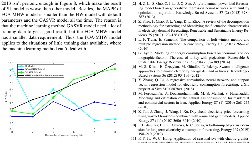
Reducing the training window from eight years to three leaves FOA-MHW near 3.58% MAPE, while the default-parameter Holt-Winters and GASVR errors rise as data shrink.
The method inherits the low data requirement of Holt-Winters and adds only a bounded optimization search, so it can be deployed where machine-learning baselines lack sufficient training samples.
The reported results apply to bimonthly series with six observations per year, where the multiplicative seasonal form fits the data.

Reading between the lines

Editorial extensions of the paper, not claims the author makes directly.

The paper leaves untested the standard practice of estimating Holt-Winters parameters directly from the training data by error minimization; a head-to-head test against that optimized Holt-Winters baseline would show whether the fruit fly search itself is needed.
Because only three parameters are searched, a simple grid search or coordinate descent over ($\alpha$, $\beta$, $\gamma$) might reproduce the same MAPE, which would place the value in parameter tuning rather than in the swarm heuristic.
The same tuning scheme could plausibly extend to additive or damped Holt-Winters and to monthly series with 12-point seasons, but the evidence here only covers $L=6$ bimonthly data.

Share X Bluesky LinkedIn Reddit HN

Signed reviews

No signed human review yet.

Editorial analysis

A structured set of objections, weighed in public.

Desk editor's note, referee report, and a circularity audit.

Desk Editor's Note

read the letter

The practical take: the central claim that FOA-MHW always beats the benchmarks is not supported, because the key Holt-Winters baseline uses fixed arbitrary parameters (α=0.2, β=0.1, γ=0.6) instead of standard optimized parameters. The paper never compares against a properly fitted Holt-Winters model, so the reported gains likely just reflect the value of tuning, not the specific optimizer. The stress-test note is right, and the paper's own Section 3.3 undermines the 'always' wording by showing the SI model does better below five years of training data.

What is actually new: applying fruit fly optimization to select Holt-Winters smoothing parameters, with two real-data case studies and a small-sample analysis. That combination may be new, and the idea is reasonable. The paper is clearly structured, and the authors are honest that the data is proprietary and that the SI model beats them in one regime, even if the conclusion overstates it.

Soft spots beyond the baseline: the FOA equations in Section 2.3 are internally inconsistent. Equations (24)-(26) define D_i = 1/sqrt(...), then S_i = 1/D_i, which gives S_i = sqrt(...), not a value in [0,1] as required for smoothing parameters. This makes the algorithm as written impossible to reproduce. There are only six test points per series, no significance tests or intervals, and no code or data. These are real problems, but the tuning idea is salvageable.

The paper is not a waste of desk space. It tackles a practical problem and the empirical setup, apart from the weak baseline, is reasonable. But as it stands, the evidence does not support the headline claims, and the algorithm description needs fixing.

For peer review: yes, send it out, but expect heavy revision. A referee should demand a comparison against standard optimized Holt-Winters (e.g., via maximum likelihood or grid search), rolling-origin evaluation, corrected equations, and ideally shared data or code. I would not cite it in current form, but it is worth a serious look as an applied contribution.

The reader's REJECT verdict is fair in substance; the paper is not publishable as-is. But the idea is not bad, and with the right comparisons it could become a legitimate applied paper.

Referee Report

4 major / 5 minor

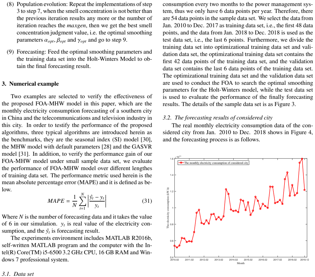
Summary. The paper proposes a hybrid forecasting model, FOA-MHW, which uses the fruit fly optimization algorithm (FOA) to select the three smoothing parameters (α, β, γ) of the multiplicative Holt-Winters (MHW) exponential smoothing method. The model is applied to monthly electricity consumption data from a Chinese city and from a telecommunications/television industry subsector, using a bimonthly reporting frequency that yields six data points per year and 54 points total (2010–2018). The data are split so that the first 42 points are used for optimization and the last 6 points of the training period (2017) serve as a validation set; the test set is the full year 2018. The authors compare FOA-MHW against a seasonal index (SI) model, an MHW model with fixed default parameters (α=0.2, β=0.1, γ=0.6), and a genetic-algorithm-tuned support vector regression (GASVR) model. They report MAPE values of 3.65% and 1.89% for FOA-MHW on the two series versus 4.38%/9.05% (SI), 4.52%/3.18% (MHW-default), and 7.00%/2.71% (GASVR). They also vary the training length down to 3 years and claim that FOA-MHW remains accurate, with a MAPE of 3.58% in the 3-year case. The paper concludes that FOA-MHW 'always achieve the best performance' over the selected benchmarks.

Significance. If the central claim were established, the paper would offer a practical, low-data forecasting tool: automatically tuned Holt-Winters smoothing with MAPE around 2–4% on bimonthly electricity series, which would be useful for utilities with limited history. The method is clearly described and the data are real, so the work is reproducible in principle. However, the significance is substantially undercut by two evidentiary weaknesses. First, the primary Holt-Winters baseline uses hand-fixed default parameters rather than a conventionally optimized Holt-Winters model, so the reported gains may reflect the value of parameter tuning rather than any special property of FOA. Second, the evaluation rests on only six test points per series, with no uncertainty quantification or significance testing, and the paper's own small-sample experiment (Figure 12) shows the SI model outperforming FOA-MHW below five years of training data, contradicting the unqualified 'always' claim. The paper thus provides a promising algorithmic idea and a plausible result, but the evidence as presented is not sufficient for the strength of the conclusions.

major comments (4)

[Section 3.2, step 3 and Tables 1–2] The primary Holt-Winters baseline, MHW with default parameters (α=0.2, β=0.1, γ=0.6), is not a standard Holt-Winters implementation. Standard practice estimates the smoothing parameters from the data, for example by minimizing one-step-ahead squared error or likelihood, as covered by the paper's own reference [28]. The reported MAPE differences between FOA-MHW and MHW-default (3.65% vs 4.52% in Table 1; 1.89% vs 3.18% in Table 2) conflate the FOA optimizer with the act of tuning parameters. To support the claim that FOA provides an advantage over standard Holt-Winters, the authors must add a benchmark that is optimized by a conventional method (e.g., grid search or likelihood maximization) on the same training/validation split, and show that FOA-MHW is at least as accurate as that benchmark.
[Section 3.1, Tables 1–2, and Section 3.3] The evaluation uses only six test points per series (the year 2018, with bimonthly data), and no confidence intervals, significance tests, or repeated subsampling are reported. The observed MAPE differences (e.g., 3.65% vs 4.52% in Table 1) may not be statistically meaningful, and the conclusion that FOA-MHW 'always achieve the best performance' is internally contradicted by Section 3.3, where the SI model is reported to have the smallest MAPE when the training data span fewer than five years (Figure 12). Please add uncertainty quantification and rephrase the conclusion to reflect the conditions under which FOA-MHW actually wins.
[Section 2.3, step 4, and Section 3.2] The FOA is a stochastic algorithm, but the paper reports only a single run with no seed information, no repeated trials, and no sensitivity analysis for the hyperparameters (sizepop=50, maxgen=20, FR=[5,10]). The reported optimal smoothing parameters (e.g., α=0.5562, β=0.2022, γ=0.3590) and the resulting MAPE values could vary substantially across runs, so the robustness of the claimed advantage is not established. Please report means and standard deviations over multiple independent runs or at least run a sensitivity analysis.
[Section 2.3, step 4, equations (21)–(26)] There is an inconsistency in the definition of the smell concentration judgment value. In the standard FOA description (equations (11)–(12)), the distance is Dist_i = sqrt(X_i^2 + Y_i^2) and S_i = 1/Dist_i. However, in step 4 of the FOA-MHW procedure, equations (24)–(26) define D_i = 1/sqrt(X_i^2 + Y_i^2), which would make S_i = 1/D_i = sqrt(X_i^2 + Y_i^2), effectively inverting the intended relation and causing the algorithm to prefer locations far from the origin. Since the paper reports convergence, this is likely a typographical error, but as written the algorithm description is not reproducible. Please correct the equations.

minor comments (5)

[Abstract] The abstract contains the typo 'the the' in the first line and several grammatical issues; please proofread throughout.
[Section 3.2 and Figure 12] In Table 1, 'July. 2018' should be 'Jul. 2018'; in Figure 12, the x-axis is drawn with the number of training years decreasing from 8 to 3, which is unconventional; consider reversing the axis order for readability.
[Introduction] The introduction states 'this is the first enhanced HW model', but there is a substantial literature on optimizing exponential smoothing parameters with metaheuristics; please soften or verify this claim with appropriate references.
[Section 2.3 and Section 3.1] The term 'optimizational training data set' is unusual; consider naming it 'fitting training set' or 'estimation set' to avoid confusion with the validation set.
[References] Reference [28] is cited for the default parameter values, but the book 'Forecasting: Methods and Applications' does not prescribe a universal default (0.2, 0.1, 0.6); please provide a precise source or state that these are arbitrary settings chosen for the baseline.

Circularity Check

0 steps flagged · score 0.0 of 10

No circular derivation: FOA parameter selection is a standard validation-block model-selection loop, and the held-out test year is not used in fitting; the paper's weaknesses are benchmark choice and an internal overclaim, not circularity.

full rationale

The FOA-MHW procedure is not circular. In Section 2.3, the FOA minimizes RMSE between Holt-Winters forecasts and the validation data set, which is defined in Section 3.1 as the last six points of the training data (months 43-48), while the test data set is the separate year 2018 (months 49-54). The optimal smoothing parameters are then fed back into the Holt-Winters recursions with the training data to produce the test forecasts. Nothing in this loop uses the test values as an input, and the final MAPE is not optimized directly; it is measured out-of-sample. The comparison against MHW with fixed defaults (alpha=0.2, beta=0.1, gamma=0.6) is a weak benchmark choice because standard practice estimates these parameters from data, and the conclusion that FOA-MHW 'always achieve the best performance' is contradicted by the paper's own Figure 12, where the SI model has the smallest MAPE for fewer than five years of training data. These are external-validity and internal-consistency concerns, not cases where a prediction reduces to its fitting input by construction.

Assumptions & free parameters 3 free parameters · 4 assumptions · 0 invented entities

The central claim rests on standard exponential smoothing recurrences, on the appropriateness of the multiplicative seasonal form for bimonthly electricity data, and on the assumption that FOA with hand-picked hyperparameters finds good smoothing parameters from the validation block. The alpha, beta, and gamma values are fitted on data, and the seasonal period and FOA settings are chosen by hand. No new entities are introduced.

free parameters (3)

Holt-Winters smoothing parameters alpha, beta, gamma = city: 0.5562, 0.2022, 0.3590; telecom: 0.7992, 0.3556, 0.9893
Chosen by FOA on the validation block and used to produce all FOA-MHW forecasts.
Seasonal period L = not stated (likely 6 for bimonthly data)
The MHW recurrence requires L, but the paper never specifies its value for the case studies, making replication ambiguous.
FOA hyperparameters (sizepop, maxgen, FR, initial range) = 50, 20, [5,10], [0,1]
Hand-chosen in Section 3.2 step (2) with no sensitivity analysis; the stated flight range is inconsistent with the reported optimal parameters.

assumptions (4)

domain assumption Multiplicative Holt-Winters recurrences (Eqs. 2-4) describe level, trend, and seasonality of the electricity series.
Used as the base model in Section 2.1; no model-selection evidence such as AIC or residual diagnostics is given.
domain assumption The seasonal component is periodic with fixed period L over the whole sample.
Needed by the MHW initialization and forecasting equations; not checked against the data and L is not stated.
domain assumption FOA converges to good smoothing parameters within the configured maxgen with a single validation split.
The paper presents convergence plots in Figures 6 and 10 but no repeated runs or statistical guarantee; results may depend on the random seed.
domain assumption The last six points of the training window are a representative validation set, and the single 2018 test year represents future conditions for every training length.
Section 3.1 defines the split 42/6/6, and Section 3.3 varies training length without rolling-origin evaluation.

how reviews work

0 comments

Cite this review

Pith. "Pith review of Monthly electricity consumption forecasting by the fruit fly optimization algorithm enhanced Holt-Winters smoothing method." pith.science (2026). https://pith.science/paper/YEJXL4FO

@misc{pith2026190806836,
  author       = {Pith},
  title        = {Pith review of: Monthly electricity consumption forecasting by the fruit fly optimization algorithm enhanced Holt-Winters smoothing method},
  year         = {2026},
  howpublished = {\url{https://pith.science/paper/YEJXL4FO}},
  note         = {Machine review of arXiv:1908.06836}
}

read the original abstract

The electricity consumption forecasting is a critical component of the intelligent power system. And accurate monthly electricity consumption forecasting, as one of the the medium and long term electricity consumption forecasting problems, plays an important role in dispatching and management for electric power systems. Although there are many studies for this problem, large sample data set is generally required to obtain higher prediction accuracy, and the prediction performance become worse when only a little data is available. However, in practical, mostly we experience the problem of insufficient sample data and how to accurately forecast the monthly electricity consumption with limited sample data is a challenge task. The Holt-Winters exponential smoothing method often used to forecast periodic series due to low demand for training data and high accuracy for forecasting. In this paper, based on Holt-Winters exponential smoothing method, we propose a hybrid forecasting model named FOA-MHW. The main idea is that, we use fruit fly optimization algorithm to select smoothing parameters for Holt-Winters exponential smoothing method. Besides, electricity consumption data of a city in China is used to comprehensively evaluate the forecasting performance of the proposed model. The results indicate that our model can significantly improve the accuracy of monthly electricity consumption forecasting even in the case that only a small number of training data is available.

Figures

Figures reproduced from arXiv: 1908.06836 by the authors.

**Figure 2.** The flowchart of FOA selecting smoothing parameter [PITH_FULL_IMAGE:figures/full_fig_p004_2.png] view at source ↗

**Figure 4.** The monthly electricity consumption of considere [PITH_FULL_IMAGE:figures/full_fig_p005_4.png] view at source ↗

Figures from the paper (7 more)

**Figure 3.** Figure 3: The details of the sample data set. The sample data set is provided by a Chinese energy supply company, which includes the monthly electricity consumption of a southern city in China from Jan. 2010 to Dec. 2018 and the monthly electricity consumption of the telecommuni…

**Figure 5.** Figure 5: The search route of fruit fly swarm for α, β and γ for the considered city. 0 5 10 15 20 25 30 35 40 The evolutional generation of furit fly population 0 0.2 0.4 0.6 0.8 1 1.2 1.4 1.6 1.8 2 The optimal smoothing parameters alpha beta gama [PITH_FULL_IMAGE:figures/full…

**Figure 6.** Figure 6: The update process of optimal smoothing parameter [PITH_FULL_IMAGE:figures/full_fig_p006_6.png]

**Figure 11.** Figure 11: The forecasting results of telecommunications a [PITH_FULL_IMAGE:figures/full_fig_p007_11.png]

**Figure 9.** Figure 9: The search route of fruit fly swarm for α, β and γ of telecommunications and television industry. 0 5 10 15 20 25 30 35 40 The evolutional generation of fruit fly population 0.2 0.4 0.6 0.8 1 1.2 1.4 1.6 1.8 2 The optimal parameters alpha beta gama [PITH_FULL_IMAGE:f…

**Figure 10.** Figure 10: The update process of optimal smoothing paramete [PITH_FULL_IMAGE:figures/full_fig_p007_10.png]

**Figure 12.** Figure 12: The MAPE of different models in different lengthes of training data in telecommunications and television industry. 4. Conclusion In this paper, we deal with the problem of accurate monthly electricity consumption forecasting. In more detail, a new hybrid forecasting …

Discussion (0). Continue with ORCID to comment.

Reference graph

Works this paper leans on

31 extracted references · 31 canonical work pages

[28]

Makridakis, S

S. Makridakis, S. C. Wheelwright, V . E. McGee, Forecast ing: methods and applications., New Y ork: Wiley, 1998 (1998)

work page 1998
[1]

K. B. Debnath, M. Mourshed, Forecasting methods in energ y planning models, Renewable and Sustainable Energy Reviews 88 (2018) 297–325 (2018)

work page 2018
[2]

H. Z. Li, S. Guo, C. J. Li, J. Q. Sun, A hybrid annual power lo ad forecast- ing model based on generalized regression neural network wi th fruit ﬂy optimization algorithm, Knowledge-Based Systems 37 (2) (2 013) 378– 387 (2013)

work page 2013
[3]

Z. Shao, F. Chao, S. L. Y ang, K. L. Zhou, A review of the deco mposition methodology for extracting and identifying the ﬂuctuation characteristics in electricity demand forecasting, Renewable and Sustainable Energy Re- views 75 (2017) 123–136 (2017)

work page 2017
[4]

L. F. Tratar, E. Strmcnik, The comparison of holt-winter s method and multiple regression method: A case study, Energy 109 (2016) 266–276 (2016)

work page 2016
[5]

G. Aydin, Modeling of energy consumption based on econom ic and de- mographic factors: The case of turkey with projections, Ren ewable & Sustainable Energy Reviews 35 (35) (2014) 382–389 (2014)

work page 2014
[6]

M. S. KIran, E. ¨Ozceylan, M. G¨ und¨ uz, T. Paksoy, Swarm intelligence approaches to estimate electricity energy demand in turkey , Knowledge- Based Systems 36 (2012) 93–103 (2012)

work page 2012
[7]

A Regressive Convolution Neural network and Support Vector Regression Model for Electricity Consumption Forecasting

Y . Zhang, Q. Li, A regressive convolution neural network and support vector regression model for electricity consumption forec asting, arXiv preprint arXiv:1810.08878v1 (2018)

work page Pith review arXiv 2018

Show all 31 references

[8]

Forouzanfar, A

M. Forouzanfar, A. Doustmohammadi, M. B. Menhaj, S. Hasa nzadeh, Modeling and estimation of the natural gas consumption for r esidential and commercial sectors in iran, Applied Energy 87 (1) (2010) 268–274 (2010)

2010
[9]

Z. Tan, J. Zhang, J. Wang, J. Xu, Day-ahead electricity pr ice forecasting using wavelet transform combined with arima and garch model s, Applied Energy 87 (11) (2010) 3606–3610 (2010)

2010
[10]

F. L. da Silva, F. L. C. Oliveira, R. C. Souza, A bottom-up bayesian exten- sion for long term electricity consumption forecasting, Energy 167 (2019) 198–210 (2019)

2019
[11]

F. Y . Ju, W. C. Hong, Application of seasonal svr with cha otic gravita- tional search algorithm in electricity forecasting, Appli ed Mathematical Modelling 37 (23) (2013) 9643–9651 (2013)

2013
[12]

J. F. Chen, Q. Do, T. Nguyen, T. Doan, Forecasting monthl y electricity de- mands by wavelet neuro-fuzzy system optimized by heuristic algorithms, Information 9 (3) (2018) 51 (2018)

2018
[13]

Hernandez, C

L. Hernandez, C. Baladron, J. M. Aguiar, B. Carro, J. Mas sana, A survey on electric power demand forecasting: Future trends in smar t grids, mi- crogrids and smart buildings, IEEE Communications Surveys & Tutorials 16 (3) (2014) 1460–1495 (2014)

2014
[14]

J. F. Rendon-Sanchez, L. M. de Menezes, Structural comb ination of sea- sonal exponential smoothing forecasts applied to load fore casting, Euro- pean Journal of Operational Research 275 (3) (2019) 916–924 (2019)

2019
[15]

G. J. Tsekouras, E. N. Dialynas, N. D. Hatziargyriou, S. Kavatza, A non- linear multivariable regression model for midterm energy f orecasting of power systems, Electric Power Systems Research 77 (12) (200 7) 1560– 1568 (2007)

2007
[16]

E. M. de Oliveira, F. L. Cyrino Oliveira, Forecasting mi d-long term elec- tric energy consumption through bagging arima and exponent ial smooth- ing methods, Energy 144 (2018) 776–788 (2018)

2018
[17]

Nawaz, N

S. Nawaz, N. Iqbal, S. Anwar, Modelling electricity dem and using the star (smooth transition auto-regressive) model in pakistan, En ergy 78 (2014) 535–542 (2014)

2014
[18]

Y . He, Y . Qin, S. Wang, X. Wang, C. Wang, Electricity consumption prob- ability density forecasting method based on lasso-quantile regression neu- ral network, Applied Energy 233-234 (2019) 565 – 575 (2019)

2019
[19]

M. H. Amjadi, H. Nezamabadi-Pour, M. M. Farsangi, Estim ation of elec- tricity demand of iran using two heuristic algorithms, Ener gy Conversion & Management 51 (3) (2010) 493–497 (2010)

2010
[20]

J. W. Taylor, R. Buizza, Neural network load forecastin g with weather ensemble predictions, IEEE Trans on Power Systems 17 (7) (20 02) 59– 59 (2002)

2002
[21]

M. S. Kandil, S. M. El-Debeiky, N. E. Hasanien, Long-ter m load fore- casting for fast developing utility using a knowledge-based expert system, IEEE Power Engineering Review 22 (4) (2002) 78–78 (2002)

2002
[22]

L. Tang, X. Wang, X. Wang, C. Shao, S. Liu, S. Tian, Long-t erm elec- tricity consumption forecasting based on expert predictio n and fuzzy bayesian theory, Energy 167 (2019) 1144 – 1154 (2019)

2019
[23]

J. Wang, X. Ma, W. Jie, D. Y ao, Optimization models based on gm (1, 1) and seasonal ﬂuctuation for electricity demand forecastin g, International Journal of Electrical Power & Energy Systems 43 (1) (2012) 10 9–117 8 (2012)

2012
[24]

D. Ali, M. Y ohanna, M. I. Puwu, B. M. Garkida, Long-term l oad fore- cast modelling using a fuzzy logic approach, Paciﬁc Science Review A Natural Science & Engineering (2016) S2405882316300217 (2 016)

2016
[25]

C. C. Holt, Forecasting seasonals and trends by exponen tially weighted moving averages, International Journal of Forecasting 20 ( 1) (2004) 5–10 (2004)

2004
[26]

P . R. Winters, Forecasting sales by exponentially weig hted moving aver- ages, Management Science 6 (3) (1960) 324–342 (1960)

1960
[27]

W. T. Pan, A new fruit ﬂy optimization algorithm: Taking the ﬁnancial distress model as an example, Knowledge-Based Systems 26 (2 ) (2012) 69–74 (2012)

2012
[29]

G. Cao, L. Wu, Support vector regression with fruit ﬂy op timization algo- rithm for seasonal electricity consumption forecasting, Energy 115 (2016) 734–745 (2016)

2016
[30]

J. Wang, X. Ma, J. Wu, Y . Dong, Optimization models based on gm (1,1) and seasonal ﬂuctuation for electricity demand forecastin g, International Journal of Electrical Power & Energy Systems 43 (1) (2012) 10 9 – 117 (2012)

2012
[31]

T. A. Oyehan, I. O. Alade, A. Bagudu, K. O. Sulaiman, S. O. Olatunji, T. A. Saleh, Predicting of the refractive index of haemoglob in using the hybrid ga-svr approach, Computers in Biology and Medicine 9 8 (2018) 85 – 92 (2018). 9

2018

Pith tools

Reviewed August 14, 2026 · model on record in the stance chip above.

[1] [28]

Makridakis, S

S. Makridakis, S. C. Wheelwright, V . E. McGee, Forecast ing: methods and applications., New Y ork: Wiley, 1998 (1998)

work page 1998

[2] [1]

K. B. Debnath, M. Mourshed, Forecasting methods in energ y planning models, Renewable and Sustainable Energy Reviews 88 (2018) 297–325 (2018)

work page 2018

[3] [2]

H. Z. Li, S. Guo, C. J. Li, J. Q. Sun, A hybrid annual power lo ad forecast- ing model based on generalized regression neural network wi th fruit ﬂy optimization algorithm, Knowledge-Based Systems 37 (2) (2 013) 378– 387 (2013)

work page 2013

[4] [3]

Z. Shao, F. Chao, S. L. Y ang, K. L. Zhou, A review of the deco mposition methodology for extracting and identifying the ﬂuctuation characteristics in electricity demand forecasting, Renewable and Sustainable Energy Re- views 75 (2017) 123–136 (2017)

work page 2017

[5] [4]

L. F. Tratar, E. Strmcnik, The comparison of holt-winter s method and multiple regression method: A case study, Energy 109 (2016) 266–276 (2016)

work page 2016

[6] [5]

G. Aydin, Modeling of energy consumption based on econom ic and de- mographic factors: The case of turkey with projections, Ren ewable & Sustainable Energy Reviews 35 (35) (2014) 382–389 (2014)

work page 2014

[7] [6]

M. S. KIran, E. ¨Ozceylan, M. G¨ und¨ uz, T. Paksoy, Swarm intelligence approaches to estimate electricity energy demand in turkey , Knowledge- Based Systems 36 (2012) 93–103 (2012)

work page 2012

[8] [7]

A Regressive Convolution Neural network and Support Vector Regression Model for Electricity Consumption Forecasting

Y . Zhang, Q. Li, A regressive convolution neural network and support vector regression model for electricity consumption forec asting, arXiv preprint arXiv:1810.08878v1 (2018)

work page Pith review arXiv 2018