The Topological Complexity of Spaces of Digital Jordan Curves

Shelley Kandola

REVIEW 3 major objections 4 minor 44 references

The Topological Complexity of Spaces of Digital Jordan Curves

T0 review · 3 major / 4 minor · reviewed 2026-08-14 · deepseek-v4-flash

Challenge this review Re-run · record.json Download PDF Read on arXiv ↗ Review JSON

Pith's one-line read The paper claims that the space of digital Jordan curves in a Khalimsky digital plane is path-connected, so a finite set of motion-planning rules can morph any segmented image into any other.

desk verdict Original and worth engaging, but the main connectivity proof leans on a lemma with gaps that need closing before Theorem 1.1 and Theorem 1.2 can be trusted. read the letter →

arxiv 1908.07015 v1 pith:WA6C4ZKN submitted 2019-08-19 math.AT cs.GR

Shelley Kandola This is my paper · ORCID

classification math.ATcs.GR MSC 55M30

keywords digitaltopologyKhalimskyJordancurvesCOTStopologicalcomplexitymotionplanningfinitespacespath-connectedness

verification ladder T0 review T1 audit T2 compute T3 formal

The pith

A machine-rendered reading of the paper's core claim, the machinery that carries it, and where it could break.

The reading

This paper claims that the collection of all digital Jordan curves in a sufficiently large Khalimsky digital plane forms a path-connected finite topological space, $J(D)$. If that is right, the topological complexity $TC(J(D))$ is finite: a finite list of continuous motion-planning rules is enough to transform any Jordan-curve-segmented image into any other. The proof has two steps: every Jordan curve can be shrunk through homotopies to a minimal Jordan curve surrounding one of its pure interior points, and any two minimal Jordan curves are connected by a fence of homotopies. The paper also claims that the Khalimsky topology is the only digital topology among those it considers for which the space of Jordan curves is path-connected.

What carries the argument

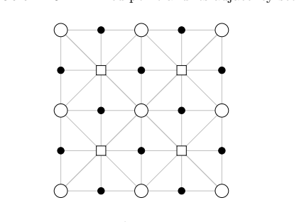
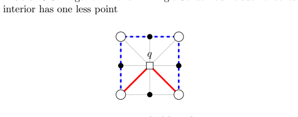
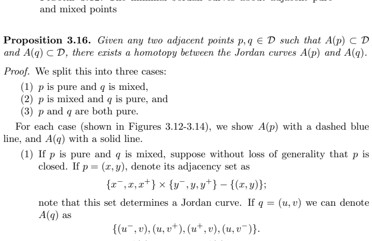
The central object is the finite $T_0$ space $J(D)$ of COTS-Jordan curves in a Khalimsky digital plane, where a COTS (connected ordered topological space) is a finite model of a line segment with alternating open and closed points. The space is given a topology through the pointwise order on $S^1$-parameterizations of curves, which recovers the compact-open topology on the mapping space. The load-bearing mechanism is the shrink algorithm: fixing a pure interior point $p$, choose $q$ of maximal COTS-distance from $p$ inside the interior; Lemma 3.8 guarantees that $A(q)\cap J$ is connected and has at least three points, which allows replacing a segment of $J$ by $q$ to produce a smaller Jordan curve homotopic to the original. Iterating reaches a minimal Jordan curve, and Proposition 3.16 supplies homotopies between minimal curves, yielding the fence that proves path-connectedness.

What would settle it

Search exhaustively through all Jordan curves of a small Khalimsky digital plane, e.g. $5\times5$ or $6\times6$, for a non-minimal $J$ and a pure $p\in\operatorname{Int}(J)$ such that some $q$ maximizing $d_{\operatorname{Int}(J)}(p,q)$ has $A(q)\cap J$ disconnected or of size $1$ or $2$; one such example would disprove Lemma 3.8 and with it Theorem 1.1.

Watch

Extended reading notes

Core claim

On the paper's own terms, the central discovery is Theorem 1.1: for a sufficiently large digital plane $D$ equipped with the Khalimsky topology, the space $J(D)$ of digital Jordan curves, topologized through the pointwise order on their standard $S^1$-parameterizations, is path-connected. A path in $J(D)$ is a finite fence of homotopies, so any two Jordan curves are connected by a sequence of continuous deformations that stay inside $J(D)$; consequently $TC(J(D))$ is finite. The path is constructed algorithmically: shrink a given curve to a minimal curve $A(p)$ around a pure interior point $p$, then move between minimal curves by the homotopies of Proposition 3.16. Theorem 1.2 states that this path-connectedness fails for the Marcus-Wyse topology and for the alternative digital topologies considered, so the Khalimsky topology is the unique one among them that supports the morphing picture.

Load-bearing premise

The proof rests on Lemma 3.8, which says that from a fixed pure interior point, a farthest interior point $q$ must meet the Jordan curve in a connected set of at least three adjacent points; if that structural fact fails for some curve, the shrinking step cannot produce a smaller homotopic Jordan curve and the path-connectedness proof collapses.

Editorial extensions

If this is right

For any sufficiently large Khalimsky digital plane, $TC(J(D))$ is finite, so a finite set of local motion-planning rules suffices to morph any Jordan-curve-segmented image into any other.
Every digital Jordan curve is homotopic to a minimal Jordan curve around one of its pure interior points, and the interior of every Jordan curve is weakly contractible.
The space of minimal Jordan curves is contractible, and for the $4\times4$ and $5\times5$ digital planes the full space $J(D)$ is contractible with $TC(J(D))=1$.
Under the Marcus-Wyse topology and the other alternative digital topologies considered, the corresponding space of digital Jordan curves is not path-connected, which the paper takes as evidence that the Khalimsky topology is the topologically correct setting.
The exact count of Jordan curves in a $3\times n$ digital plane is $(n-1)(n-2)/2$, and the maximal and minimal elements of $J(D)$ correspond to polyominoes, giving combinatorial bounds on the size and complexity of the space.

Reading between the lines

Editorial extensions of the paper, not claims the author makes directly.

The shrink algorithm itself is an explicit motion planner: it produces a path between any two Jordan curves whose length is controlled by the size of the interior, so a practical morphing pipeline could be built directly from the proof rather than from an abstract section of the path space.
The same parameterize-and-shrink strategy might extend to digital 3-space, where the analogue of Lemma 3.8 would need a surface-adjacency condition; a failure there would mark a genuine boundary of the method.
The polyomino correspondence suggests that the number of maximal elements of $J(D)$ grows rapidly with the plane, so the finite value of $TC(J(D))$ is likely to be large even for modest image sizes.
A finite-space version of efficient topological complexity that minimizes height travelled in the Hasse diagram could turn the theorem into motion planners that produce visually intuitive morphs.

Share X Bluesky LinkedIn Reddit HN

Signed reviews

No signed human review yet.

Editorial analysis

A structured set of objections, weighed in public.

Desk editor's note, referee report, and a circularity audit.

Desk Editor's Note

read the letter

Sam—quick take on Kandola, 1908.07015. The genuinely new thing is the setup: treating the set of COTS-Jordan curves in a Khalimsky plane as a finite space, with topological complexity as a measure of image-morphing cost. That is a real idea, and the paper makes it concrete with explicit parameterizations and a shrinking algorithm. The small-plane census and the link to Tanaka's combinatorial complexity give useful data. The novelty is not dressed-up old machinery.

What is good: the path-connectedness claim comes with an explicit iterative shrink-to-minimal curve, and the minimal-curve homotopies in Proposition 3.16 are worked through by hand. The paper also honestly flags places where it is guessing, notably the converse of Proposition 3.22 and contractibility of interiors.

The soft spots are real. Lemma 3.8 is load-bearing, and its proof has gaps. The stress-test note is right: part (a) asserts that a_{n-1} and b both have distance n-1 from p, but the text only forces b to have distance n-1 or n, and if n then the maximality contradiction does not go through. The step where the construction is repeated over all choices of j0 until b lands in the right region is asserted, not argued. Part (c) states that an adjacent pure point has distance n-2 when adjacency would force distance at least n-1; a parity argument probably repairs it, but that repair is absent. The homotopy step in Theorem 3.15 also needs more care: for pure q, comparability works globally, but for mixed q the proof checks only the single replaced point and then claims g and f are comparable everywhere.

Theorem 1.2 has its own problems. The wedge-of-circles count has a sign issue, and the claim that distinct Jordan curves give distinct homology classes in the wedge is asserted without proof. The strong conclusion that Khalimsky is the only topologically correct digital topology is not established at the paper's current level of rigor. The 5x5 enumeration is hand-drawn and should be machine-checked before anyone relies on it.

Who is this for: people working in digital topology, finite spaces, or topological complexity. The core idea is sound enough that I would send it to peer review, but I would insist on a repaired Lemma 3.8, a tightened homotopy argument in Theorem 3.15, and verification of the enumerations before publication.

Referee Report

3 major / 4 minor

Summary. The paper defines the space J(D) of all digital Jordan curves in a finite Khalimsky digital plane as a finite T0 topological space, using S1-parameterizations and the pointwise order on maps. The central claim is Theorem 1.1, that J(D) is path-connected, which would imply that the unreduced topological complexity TC(J(D)) is finite. The proof strategy is to show via an explicit shrinking algorithm that every Jordan curve can be connected by a fence of homotopies to a minimal Jordan curve about one of its pure interior points (Theorem 3.15), and then to connect minimal Jordan curves by explicit homotopies (Proposition 3.16). The paper also proves auxiliary results on COTS-distance in finite spaces, claims Theorem 1.2 that among several digital topologies only the Khalimsky topology makes J(D) path-connected, and gives enumerations and topological-complexity computations for small digital planes.

Significance. If the central results hold, this is an original and potentially useful contribution: it treats digital images as points in a configuration space and connects image morphing to topological complexity. The paper contains explicit algorithms (Algorithm 3.6), explicit homotopies between minimal Jordan curves, and useful auxiliary facts about COTS-distance such as Proposition 2.11 and Proposition 2.12. It also gives concrete small-plane enumerations that are valuable for testing conjectures. The main weakness is that the proof of the load-bearing structural lemma, Lemma 3.8, contains substantial unjustified steps, and the proof of Theorem 1.2 contains a graph-theoretic assertion that is not valid as stated. With repaired proofs, the paper would be a meaningful contribution to digital topology and finite-space topological complexity.

major comments (3)

[§3.1, Lemma 3.8(a)] This is the structural fact on which the Shrink step of Theorem 3.15 depends, and its proof is not complete. After constructing β=β'∪{q}, the text asserts that 'a_{n−1} and b are both of distance n−1 from p.' For a_{n−1} this follows from Proposition 2.7, but for b the preceding argument only gives b∈A(q)−J and, in the branch under consideration, that a shortest arc from p to b does not run through q. This does not force d(p,b)=n−1; d(p,b)=n is possible, in which case β is a p-to-q path of length n+1 and the claimed contradiction with maximality does not apply. The proof also contains the existence assertion 'By performing this construction for every choice of j0, we will eventually arrive at a choice of j0 such that b∈(A(q)−J)∩Int(K),' with no argument that some choice works. The companion assertion that a_{n−1} lies in Ext(K)∩Int(J) is likewise not derived from the construction. Since Lemma 3.8 is the input that guarantees |A(q)∩J|≥3 and hence that Shrink produces a smaller Jordan curve, the proof of Theorem 3.15 and therefore of Theorem 1.1 is incomplete as written.
[§3.1, Lemma 3.8(c)] The final inequality in part (c) is misstated. The text says that if a point of A(q) has distance n−2 from p, then 'd(p,q)=n−1<n, a contradiction.' What follows is only d(p,q)≤n−1, not equality. This is enough to contradict the choice of q as a point of maximal distance n, provided one uses the inequality rather than the displayed equality. The repair is local, but as written the sentence contains a false assertion inside the proof of a key lemma.
[§4.1, proof of Theorem 1.2] The proof that no path exists between distinct Jordan curves in a non-Khalimsky T_{1/2} digital plane relies on the assertion that two distinct 1-chains outside a spanning tree determine different homotopy classes in the wedge of circles. This is not valid in general: in a graph-thickened digital plane, distinct simple cycles can be homologous (e.g., the two bounding cycles of a theta-shaped subgraph), so the displayed comparison of the chosen 1-chains does not imply that |K(f)| and |K(f')| lie in different classes of π1. The argument would need to compare the actual 1-cycles, not just a single outside edge for each curve. As written, Theorem 1.2 is therefore unproved. There is also a sign issue in the same proof: for a connected graph the number of circles in a wedge decomposition is 1−χ(D), not χ(D)−1.

minor comments (4)

[§3.2, Theorem 3.15, step (3)] The sentence 'but q∉Int(J)' is false because q is chosen in Int(J); the intended statement is that q∉Int(K) for the new Jordan curve K.
[§2.1, Proposition 2.3] The proof of Proposition 2.3 would benefit from a precise definition of the 'loop' and of the elimination procedure; as written, the existence of the lowest index i and the verification that the resulting set is a COTS-arc are only sketched.
[Throughout] There are numerous spelling and typographical errors that should be corrected in revision, for example 'conntected', 'Futhermore', 'reperesent', and 'worth nothing' for 'worth noting'.
[§3.3] The notation 'J1(D)' for the space of minimal Jordan curves is introduced and used before the subsection where it is formally defined; consider defining it earlier for readability.

Circularity Check

0 steps flagged · score 0.0 of 10

No significant circularity: the paper's derivations are self-contained and its central results do not reduce to fitted inputs or self-citations.

full rationale

The paper's central results are derived from stated definitions and externally established theorems rather than from a self-referential chain. Theorem 1.1, path-connectedness of J(D), is obtained by combining Lemma 3.8, the shrinking algorithm of Theorem 3.15, and Proposition 3.16, each of which is proved from the Khalimsky plane axioms, COTS properties, Stong's finite-space theorems, McCord's weak equivalences, and the Jordan curve theorem of [27]. There is no fitted parameter later renamed as a prediction, and no definition of a central object in terms of the theorem it is used to prove. The only self-citation is to the author's earlier work [24], and it appears as motivation and as one of two independent references for a general inequality cat(X×X) ≤ cat(X)^2; this citation is not load-bearing for Theorem 1.1 or Theorem 1.2. Theorem 1.2 is proved by explicit comparison with the three non-Khalimsky topologies reviewed in Section 1.3.2, and the argument does not assume the conclusion. The paper even records an admitted limitation: 'We conjecture that the converse of Proposition 3.22 is true, however, this has yet to be shown.' Skeptical concerns about Lemma 3.8 concern possible gaps in a specific proof, not a circular reduction; no equation in the paper reduces to its own input, and no predicted quantity is forced by construction. Therefore the circularity score is 0.

Assumptions & free parameters 0 free parameters · 8 assumptions · 0 invented entities

No free parameters are fitted; the paper uses only the structure of finite Khalimsky planes and standard theorems of finite-space topology. The axioms listed are the external results and domain assumptions the central proofs rely on. The paper does not introduce new physical entities.

assumptions (8)

standard math Continuity between finite T0 spaces is equivalent to order-preserving maps (Stong, Proposition 7 of [39]).
Used throughout to convert homotopies and the pointwise order on J(D) into topological statements.
standard math Contractibility of a finite T0 space is detected by its core being a single point (Stong, Corollary 4 of [39]).
Used to show COTS products and J(D4x4) are contractible.
standard math The McCord map gives a weak homotopy equivalence between a finite space and its order complex (McCord [33]).
Used in Section 4.1 to compute the fundamental group of non-Khalimsky digital planes from their order complexes.
domain assumption Khalimsky-Kopperman-Meyer digital Jordan curve theorem: the complement of a COTS-Jordan curve has exactly two components (Theorem of [27]).
Defines interior and exterior of digital Jordan curves; used in Lemmas 3.3, 3.8, Proposition 3.7, and the shrinking algorithm.
standard math The COTS-distance function d is a metric (Proposition 2.5).
Proved in the paper; the metric property underlies the distance arguments in Lemma 3.8 and the algorithm's maximal-distance choice.
domain assumption The digital plane D is sufficiently large so that chosen interior points have full adjacency sets and border effects do not occur.
Used without quantitative bounds in Theorem 3.15 and Proposition 3.16; results could fail for small planes if a maximal-distance point lies near the border.
domain assumption The order complex of a T_{1/2} digital plane with height-one Hasse diagram is a graph homotopy equivalent to a wedge of circles (derived from Remark 3.3.1 of [3]).
Used in the proof of Theorem 1.2 to show non-Khalimsky planes have nontrivial fundamental group; the paper misstates the number of circles and does not prove the wedge decomposition itself.
domain assumption Distinct simple cycles in a graph model of a digital plane represent distinct homotopy classes in the wedge-of-circles fundamental group.
Used in the proof of Theorem 1.2 to conclude that distinct Jordan curves are not homotopic; no proof or reference is supplied.

how reviews work

0 comments

Cite this review

Pith. "Pith review of The Topological Complexity of Spaces of Digital Jordan Curves." pith.science (2026). https://pith.science/paper/WA6C4ZKN

@misc{pith2026190807015,
  author       = {Pith},
  title        = {Pith review of: The Topological Complexity of Spaces of Digital Jordan Curves},
  year         = {2026},
  howpublished = {\url{https://pith.science/paper/WA6C4ZKN}},
  note         = {Machine review of arXiv:1908.07015}
}

abstract

This research is motivated by studying image processing algorithms through a topological lens. The images we focus on here are those that have been segmented by digital Jordan curves as a means of image compression. The algorithms of interest are those that continuously morph one digital image into another digital image. Digital Jordan curves have been studied in a variety of forms for decades now. Our contribution to this field is interpreting the set of digital Jordan curves that can exist within a given digital plane as a finite topological space. Computing the topological complexity of this space determines the minimal number of continuous motion planning rules required to transform one image into another, and determining the motion planners associated to topological complexity provides the specific algorithms for doing so. The main result of Section 3 is that our space of digital Jordan curves is connected, hence, its topological complexity is finite. To build up to that, we use Section 2 to prove some results about paths and distance functions that are obvious in Hausdorff spaces, yet surprisingly elusive in $T_0$ spaces. We end with Section 4, in which we study applications of these results. In particular, we prove that our interpretation of the space of digital Jordan curves is the only topologically correct interpretation. This article is an adaptation of the author's Ph.D. dissertation.

Figures

Figures reproduced from arXiv: 1908.07015 by the authors.

**Figure 1.1.** The commutative diagram for TC (X) Definition 1.5. The Schwarz genus g(p) of a fibration p : E → B is the minimal number k such that there exists an open covering U1, . . . , Uk of B where each set Ui admits a local p-section. That is, each Ui has an associated map si such that p ◦ si ' 1B. Consider [PITH_FULL_IMAGE:figures/full_fig_p006_1_1.png] view at source ↗

**Figure 1.2.** The Hasse diagram of a COTS with 9 points Theorem 3.2 of [40] proves the following: It holds that TC (X) = CC(X) for any connected finite space X. Because connected finite spaces are path-connected by Proposition 1.2.4 of [3], this is sufficient for defining a notion of topological complexity. In Example 4.5 of that paper, Tanaka proves that for the minimal finite model S 1 of S 1 , TC S 1 = 4; this is the result … view at source ↗

**Figure 1.3.** cots A finite COTS X with the minimal open set of each point circled component of X − {y}. As subspaces of Y − {y}, each of {x} and {z} are open. Within Y , the open sets are {x} or {x, y} along with {z} or {y, z}. Note that {x}, {y}, and {z} cannot all be open sets of Y , or else Y would have the discrete topology, and Y would not be connected. So there are four cases to consider. If the open sets of Y are {x} and … view at source ↗

Figures from the paper (40 more)

**Figure 1.** Figure 1: or Figure 1.5. If [PITH_FULL_IMAGE:figures/full_fig_p010_1.png]

**Figure 1.4.** Figure 1.4: An open point and its adjacency set [PITH_FULL_IMAGE:figures/full_fig_p011_1_4.png]

**Figure 1.5.** Figure 1.5: A closed point and its adjacency set [PITH_FULL_IMAGE:figures/full_fig_p011_1_5.png]

**Figure 1.6.** Figure 1.6: A mixed point and its adjacency set [PITH_FULL_IMAGE:figures/full_fig_p011_1_6.png]

**Figure 1.7.** Figure 1.7: A 5 × 5 digital plane 1.7 or its dual, depending on whether the endpoints of X are open or closed. For example, if X is the COTS in [PITH_FULL_IMAGE:figures/full_fig_p011_1_7.png]

**Figure 1.9.** Figure 1.9: A COTSarc that is a subset of the COTS-path in [PITH_FULL_IMAGE:figures/full_fig_p012_1_9.png]

**Figure 1.** Figure 1: shows a mapping of a finite COTS into [PITH_FULL_IMAGE:figures/full_fig_p012_1.png]

**Figure 1.10.** Figure 1.10: A subset of Z 2 with the Marcus-Wyse topology to topologize the integers in such a way that the connected sets are the sets of consecutive integers? Generalize to the lattice points of n-space.” In this context, two points in Z n are “consecutive” if they differ by …

**Figure 1.11.** Figure 1.11: A tile of the connectedness graph of (Z 2 , w) [PITH_FULL_IMAGE:figures/full_fig_p015_1_11.png]

**Figure 1.12.** Figure 1.12: A tile of the connectedness graph of (Z 2 , wˆ) [PITH_FULL_IMAGE:figures/full_fig_p015_1_12.png]

**Figure 1.13.** Figure 1.13: The 6-neighbors of a point in Z 2 This fails to be a topology because (7, 4) 6∈ u(6, 2) 6= u(u(6, 2)) 3 (7, 4), for example. In [34] and [11], they discuss the possibility of a 6-adjacency structure on Z 2 . In such a structure, every point of Z 2 has 6 neighbors, a…

**Figure 2.1.** Figure 2.1: Neighbors of q and their coordinates Proof. Let p, q ∈ D be pure points on the same diagonal. Translate and reflect the coordinate system on D such that p = (0, 0) and q = (n, n) for some positive integer n. By Proposition 2.10, d(p, q) = n. We will prove via inducti…

**Figure 3.1.** Figure 3.1: A 3-point connected subset of D and some neighbors, for use in Example 3.4 Proof. First we show that if J is not minimal, then |Int (J)| ≥ 2. If J is not minimal, then J 6= A(p) for some p ∈ D that does not touch the border. Because Int (J) 6= ∅, |Int (J)| ≥ 1. Suppo…

**Figure 3.2.** Figure 3.2: An example of A(q) ∩ J being disconnected for q of maximal distance (a) A(q) ∩ J is connected: If A(q) ∩ J = ∅, then it is vacuously connected. Otherwise, if dq = n is maximal, and since Int (J) is arcwise-connected, there exists a (not necessarily unique) shortest C…

**Figure 3.3.** Figure 3.3: |A(q) ∩ J| = 1 and q is pure q e f c d [PITH_FULL_IMAGE:figures/full_fig_p027_3_3.png]

**Figure 3.4.** Figure 3.4: |A(q) ∩ J| = 0 and q is pure |A(jm0 ) ∩ C| > 0. Clearly, C and {j0, j1, . . . , jm0} ⊂ J are each COTS-arcs whose endpoints are adjacent. By Proposition 2.3, C ∪ {j1, j2, . . . , jm0} contains a COTS-arc C 0 as a subset that starts at j1 and ends at q. Note the omiss…

**Figure 3.5.** Figure 3.5: An application of Lemma 3.8 to a Jordan curve (in blue), with the adjacency lines of the digital plane omitted Proposition 3.13. Every digital Jordan curve admits a parametrization by S 1 . Proof. By Proposition 3.1, we can suppose |J| = n for some even integer n. De…

**Figure 3.6.** Figure 3.6: Algorithm for shrinking a Jordan curve such that its interior has one less point q [PITH_FULL_IMAGE:figures/full_fig_p031_3_6.png]

**Figure 3.7.** Figure 3.7: |A(q) ∩ J| = 7 q [PITH_FULL_IMAGE:figures/full_fig_p031_3_7.png]

**Figure 3.8.** Figure 3.8: |A(q) ∩ J| = 5 that |A(j0) ∩ K| = [PITH_FULL_IMAGE:figures/full_fig_p031_3_8.png]

**Figure 3.9.** Figure 3.9: |A(q) ∩ J| = 3 and q is pure q [PITH_FULL_IMAGE:figures/full_fig_p032_3_9.png]

**Figure 3.10.** Figure 3.10: |A(q) ∩ J| = 3 and q is mixed 1: procedure Minimalize(J, f, p) 2: if |Int (J)| = 1 then 3: return (J, f, p) 4: (K, g, p) ← (J, f, p) 5: while |Int (K)| > 1 do 6: (K, g, p) ← Shrink(K, g, p) 7: return (K, g, p) [PITH_FULL_IMAGE:figures/full_fig_p032_3_10.png]

**Figure 3.11.** Figure 3.11: Algorithm for shrinking a Jordan curve until it is minimal If q is pure, suppose without loss of generality that q is closed. Then A(q) ∩ J = q ↓ ∩ J, so q ≥ r for all r ∈ A(q) ∩ J. Then g(t) ≥ f(t) for all t ∈ f −1 (J 00), where J 00 is J 0 minus its endpoints. Sin…

**Figure 3.12.** Figure 3.12: The minimal Jordan curves about adjacent pure and mixed points Proposition 3.16. Given any two adjacent points p, q ∈ D such that A(p) ⊂ D and A(q) ⊂ D, there exists a homotopy between the Jordan curves A(p) and A(q). Proof. We split this into three cases: (1) p is …

**Figure 3.** Figure 3: displays [PITH_FULL_IMAGE:figures/full_fig_p033_3.png]

**Figure 3.13.** Figure 3.13: The minimal Jordan curves about adjacent mixed and pure points (2) If p is mixed and q is pure, suppose without loss of generality that q is closed. Assume p = (x, y) and q = (u, v), and denote their adjacency sets as above. Suppose without loss of generality that q…

**Figure 3.14.** Figure 3.14: The minimal Jordan curves about two adjacent pure points g(t) =    (u −, v−), t ∈ f −1 ((x, y−) ∪ (x −, y−) ∪ (x −, y)) (u −, v), t ∈ f −1 ((x −, y+)) (u −, v+), t ∈ f −1 ((x, y+)) (u, v+), t ∈ [PITH_FULL_IMAGE:figures/full_fig_p035_3_14.png]

**Figure 3.15.** Figure 3.15: The 4 × 4 Khalimsky digital plane another. If J ≤ K in J1(D), each are of the form A(p) and A(q), respectively. Since J1(D) ⊆ J (D) is T0, if J and K are distinct, then J < K, in fact. Then there are three cases for J = A(p) < A(q) = K: (1) p is closed and q is mixe…

**Figure 3.16.** Figure 3.16: The Hasse diagram of J (D4×4) 4. The adjusted border is also a Jordan curve, whose interior is all four points mentioned above. All in all, |J (D4×4)| = 11, and we’ve displayed the Jordan curves in [PITH_FULL_IMAGE:figures/full_fig_p040_3_16.png]

**Figure 3.17.** Figure 3.17: A continuous path between two Jordan curves given by the motion planner on a space with a maximal element Intuitively, we can see how the pointwise order topology dictates the structure of the Hasse diagram in [PITH_FULL_IMAGE:figures/full_fig_p041_3_17.png]

**Figure 3.18.** Figure 3.18: A more intuitive path than the one given in [PITH_FULL_IMAGE:figures/full_fig_p042_3_18.png]

**Figure 3.19.** Figure 3.19: Jordan curves in J (D5×5) ( [PITH_FULL_IMAGE:figures/full_fig_p044_3_19.png]

**Figure 3.20.** Figure 3.20: Jordan curves in J (D5×5) ( [PITH_FULL_IMAGE:figures/full_fig_p045_3_20.png]

**Figure 3.21.** Figure 3.21: Jordan curves in J (D5×5) ( [PITH_FULL_IMAGE:figures/full_fig_p046_3_21.png]

**Figure 3.22.** Figure 3.22: Jordan curves in J (D5×5) ( [PITH_FULL_IMAGE:figures/full_fig_p047_3_22.png]

**Figure 3.23.** Figure 3.23: The top two rows of the Hasse diagram of J (D5×5) establish a correspondence between image processing algorithms and paths in spaces of digital images. Paths in a space of digital images represent a sequence of images to pass through in navigating from one image to …

**Figure 4.1.** Figure 4.1: The geometric realization of [PITH_FULL_IMAGE:figures/full_fig_p049_4_1.png]

**Figure 4.2.** Figure 4.2: The geometric realization of [PITH_FULL_IMAGE:figures/full_fig_p049_4_2.png]

**Figure 4.3.** Figure 4.3: A wedge of 16 circles homotopy equivalent to [PITH_FULL_IMAGE:figures/full_fig_p049_4_3.png]

**Figure 4.4.** Figure 4.4: A pixelated character “7” all Jordan curves in a 16 × 16 pixel plane, some of which we might recognize as characters. Declare [PITH_FULL_IMAGE:figures/full_fig_p051_4_4.png]

Discussion (0). Continue with ORCID to comment.

Reference graph

Works this paper leans on

44 extracted references · 43 canonical work pages

[1]

M Al Hajri, Karim Belaid, and Lamia Jaafar, On khalimsky topology and applications on the digital image segmentation , Applied Mathematical Sciences 9 (2015), 3687–3701

work page 2015
[2]

Alexandroﬀ, Diskrete ra¨ ume, Rec

P.S. Alexandroﬀ, Diskrete ra¨ ume, Rec. Math. [Mat. Sbornik] N.S. 2(44) (1937), no. 3, 501— 519

work page 1937
[3]

Barmak, Algebraic topology of ﬁnite topological spaces and applications, Lecture Notes in Mathematics, vol

Jonathan A. Barmak, Algebraic topology of ﬁnite topological spaces and applications, Lecture Notes in Mathematics, vol. 2032, Springer, Heidelberg, 2011. MR 3024764

work page 2011
[4]

Gordon O. Berg, W. Julian, R. Mines, and F. Richman, The constructive Jordan curve theorem, Rocky Mountain J. Math. 5 (1975), 225–236. MR 0410701

work page 1975
[5]

Zbigniew B l aszczyk and Jos´ e Gabriel Carrasquel-Vera,Topological complexity and eﬃciency of motion planning algorithms, Rev. Mat. Iberoam. 34 (2018), no. 4, 1679–1684. MR 3896245 52 SHELLEY KANDOLA

work page 2018
[6]

Laurence Boxer, A classical construction for the digital fundamental group , J. Math. Imaging Vision 10 (1999), no. 1, 51–62. MR 1692842

work page 1999
[7]

, Properties of digital homotopy , J. Math. Imaging Vision 22 (2005), no. 1, 19–26. MR 2138582

work page 2005
[8]

Laurence Boxer and P Staecker, Homotopy relations for digital images , Note di Matematica 37 (2017), 99–126

work page 2017

Show all 44 references

[9]

3, 294 – 300

Jean-Marc Chassery, Connectivity and consecutivity in digital pictures , Computer Graphics and Image Processing 9 (1979), no. 3, 294 – 300

1979
[10]

Ulrich Eckhardt and Longin Jan Latecki, Digital topology, Digital Topology, 1994

1994
[11]

3, 295 – 312

, Topologies for the digital spaces Z2 and Z3, Computer Vision and Image Under- standing 90 (2003), no. 3, 295 – 312

2003
[12]

El-Fattah El-Atik, M

A. El-Fattah El-Atik, M. E. Abd El-Monsef, and E. I. Lashin, On ﬁnite T0 topological spaces, Proceedings of the Ninth Prague Topological Symposium (2001), Topol. Atlas, North Bay, ON, 2002, pp. 75–90. MR 1906830

2001
[13]

Michael Farber, Topological complexity of motion planning , Discrete Comput. Geom. 29 (2003), no. 2, 211–221. MR 1957228

2003
[14]

Fern´ andez-Ternero, E

D. Fern´ andez-Ternero, E. Mac´ ıas-Virg´ os, E. Minuz, and J. A. Vilches,Discrete topological complexity, Proc. Amer. Math. Soc. 146 (2018), no. 10, 4535–4548. MR 3834677

2018
[15]

Frank and E

L. Frank and E. Hubert, Pretopological approach for supervised learning, Proceedings of 13th International Conference on Pattern Recognition, vol. 4, Aug 1996, pp. 256–260 vol.4

1996
[16]

S. W. Golomb, Checker boards and polyominoes, Amer. Math. Monthly 61 (1954), 675–682. MR 0067055

1954
[17]

Jes´ us Gonz´ alez,Simplicial complexity: piecewise linear motion planning in robotics , New York J. Math. 24 (2018), 279–292. MR 3778506

2018
[18]

Methods Nonlinear Anal

Jes´ us Gonz´ alez, B´ arbara Guti´ errez, and Sergey Yuzvinsky,Higher topological complexity of subcomplexes of products of spheres and related polyhedral product spaces , Topol. Methods Nonlinear Anal. 48 (2016), no. 2, 419–451. MR 3642766

2016
[19]

MR 1867354

Allen Hatcher, Algebraic topology , Cambridge University Press, Cambridge, 2002. MR 1867354

2002
[20]

OEIS Foundation Inc., The on-line encyclopedia of integer sequences , http://oeis.org/A140517, 2019

2019
[21]

, The on-line encyclopedia of integer sequences , http://oeis.org/A118797, 2019

2019
[22]

, The on-line encyclopedia of integer sequences , http://oeis.org/A000217, 2019

2019
[23]

157 (2010), no

Norio Iwase and Michihiro Sakai, Topological complexity is a ﬁbrewise L-S category, Topology Appl. 157 (2010), no. 1, 10–21. MR 2556074

2010
[24]

Shelley Kandola, The Topological Complexity of Finite Models of Spheres , arXiv e-prints (2018), arXiv:1812.07604

2018 arXiv
[25]

˙Ismet Karaca and Melih ˙Is, Digital topological complexity numbers , Turkish J. Math. 42 (2018), no. 6, 3173–3181. MR 3885444

2018
[26]

Meyer, Boundaries in digital planes , J

Eﬁm Khalimsky, Ralph Kopperman, and Paul R. Meyer, Boundaries in digital planes , J. Appl. Math. Stochastic Anal. 3 (1990), no. 1, 27–55. MR 1051772

1990
[27]

36 (1990), no

, Computer graphics and connected topologies on ﬁnite ordered sets , Topology Appl. 36 (1990), no. 1, 1–17. MR 1062180

1990
[28]

Christer Kiselman, Digital jordan curve theorems , Digital Jordan Curve Theorems, 09 2000

2000
[29]

T. Y. Kong, A. W. Roscoe, and A. Rosenfeld, Concepts of digital topology , Topology Appl. 46 (1992), no. 3, 219–262, Special issue on digital topology. MR 1198732

1992
[30]

V.A Kovalevsky, Finite topology as applied to image analysis , Computer Vision, Graphics, and Image Processing 45 (1989), no. 2, 266

1989
[31]

Lusternik and L

L. Lusternik and L. Schnirelmann, M´ ethodes topologiques dans les probl` emmes variationnels, Actualit´ es scientiﬁques et industrielles ; 188, Hermann, Paris, 1934 (fre)

1934
[32]

10, 1119–1119

Dan Marcus and Cleveland State University Problem Solving Group, 5712, The American Mathematical Monthly 77 (1970), no. 10, 1119–1119

1970
[33]

McCord, Singular homology groups and homotopy groups of ﬁnite topological spaces, Duke Math

Michael C. McCord, Singular homology groups and homotopy groups of ﬁnite topological spaces, Duke Math. J. 33 (1966), 465–474. MR 0196744

1966
[34]

Pavel Ptak, Helmut Koﬂer, and Walter Kropatsch, Digital topologies revisited: An ap- proach based on the topological point-neighbourhood , Discrete Geometry for Computer Im- agery (Berlin, Heidelberg) (Ehoud Ahronovitz and Christophe Fiorio, eds.), Springer Berlin Heidelberg, ...

1997
[35]

Azriel Rosenfeld, Digital topology , Amer. Math. Monthly 86 (1979), no. 8, 621–630. MR 546174

1979
[36]

1, 76 – 87

Azriel Rosenfeld, Fuzzy digital topology, Information and Control 40 (1979), no. 1, 76 – 87

1979
[37]

Rudyak, On higher analogs of topological complexity , Topology Appl

Yuli B. Rudyak, On higher analogs of topological complexity , Topology Appl. 157 (2010), no. 5, 916–920. MR 2593704

2010
[38]

Punam K. Saha, Fuzzy digital topology and geometry and their applications to medical imaging, Pattern Recognition and Machine Intelligence (Berlin, Heidelberg) (Pradipta Maji, Ashish Ghosh, M. Narasimha Murty, Kuntal Ghosh, and Sankar K. Pal, eds.), Springer Berlin Heidelberg,...

2013
[39]

R. E. Stong, Finite topological spaces, 1966, pp. 325–340. MR 0195042

1966
[40]

Kohei Tanaka, A combinatorial description of topological complexity for ﬁnite spaces, Algebr. Geom. Topol. 18 (2018), no. 2, 779–796. MR 3773738

2018
[41]

153 (2006), no

Josef ˇSlapal, Digital Jordan curves , Topology Appl. 153 (2006), no. 17, 3255–3264. MR 2260583

2006
[42]

, Jordan curve theorems with respect to certain pretopologies onZ2, Discrete Geometry for Computer Imagery (Berlin, Heidelberg) (Sreˇ cko Brlek, Christophe Reutenauer, and Xavier Proven¸ cal, eds.), Springer Berlin Heidelberg, 2009, pp. 252–262

2009
[43]

A. S. ˇSvarc, The genus of a ﬁber space , Dokl. Akad. Nauk SSSR (N.S.) 119 (1958), 219–222. MR 0102812

1958
[44]

Zadeh, Fuzzy sets, Information and Control 8 (1965), no

L.A. Zadeh, Fuzzy sets, Information and Control 8 (1965), no. 3, 338 – 353

1965

Pith tools

Reviewed August 14, 2026 · model on record in the stance chip above.

[1] [1]

M Al Hajri, Karim Belaid, and Lamia Jaafar, On khalimsky topology and applications on the digital image segmentation , Applied Mathematical Sciences 9 (2015), 3687–3701

work page 2015

[2] [2]

Alexandroﬀ, Diskrete ra¨ ume, Rec

P.S. Alexandroﬀ, Diskrete ra¨ ume, Rec. Math. [Mat. Sbornik] N.S. 2(44) (1937), no. 3, 501— 519

work page 1937

[3] [3]

Barmak, Algebraic topology of ﬁnite topological spaces and applications, Lecture Notes in Mathematics, vol

Jonathan A. Barmak, Algebraic topology of ﬁnite topological spaces and applications, Lecture Notes in Mathematics, vol. 2032, Springer, Heidelberg, 2011. MR 3024764

work page 2011

[4] [4]

Gordon O. Berg, W. Julian, R. Mines, and F. Richman, The constructive Jordan curve theorem, Rocky Mountain J. Math. 5 (1975), 225–236. MR 0410701

work page 1975

[5] [5]

Zbigniew B l aszczyk and Jos´ e Gabriel Carrasquel-Vera,Topological complexity and eﬃciency of motion planning algorithms, Rev. Mat. Iberoam. 34 (2018), no. 4, 1679–1684. MR 3896245 52 SHELLEY KANDOLA

work page 2018

[6] [6]

Laurence Boxer, A classical construction for the digital fundamental group , J. Math. Imaging Vision 10 (1999), no. 1, 51–62. MR 1692842

work page 1999

[7] [7]

, Properties of digital homotopy , J. Math. Imaging Vision 22 (2005), no. 1, 19–26. MR 2138582

work page 2005

[8] [8]

Laurence Boxer and P Staecker, Homotopy relations for digital images , Note di Matematica 37 (2017), 99–126

work page 2017