REVIEW 3 major objections 5 minor 34 references
Damping Mechanisms of the Solar Filament Longitudinal Oscillations in Weak Magnetic Field
T0 review · 3 major / 5 minor · reviewed 2026-08-14 · deepseek-v4-flash
Pith's one-line read In weak magnetic fields, oscillating solar filaments leak fast-mode waves, halve their decay time, and break the pendulum-model relation between period and dip curvature — overestimating the inferred curvature radius by ~100%.
desk verdict Solid wave-leakage simulation undermined by an overstated ~100% claim that mixes thermal and deformation effects. read the letter →
The pith
A machine-rendered reading of the paper's core claim, the machinery that carries it, and where it could break.
The reading
What carries the argument
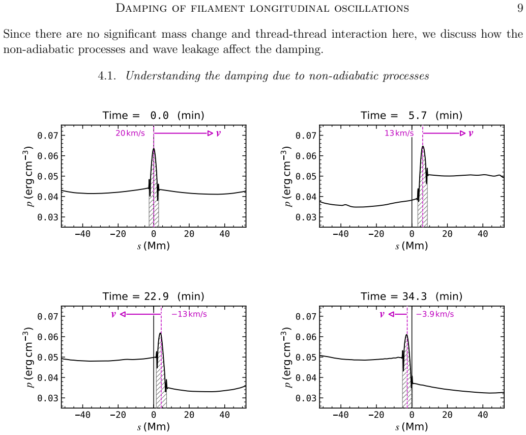
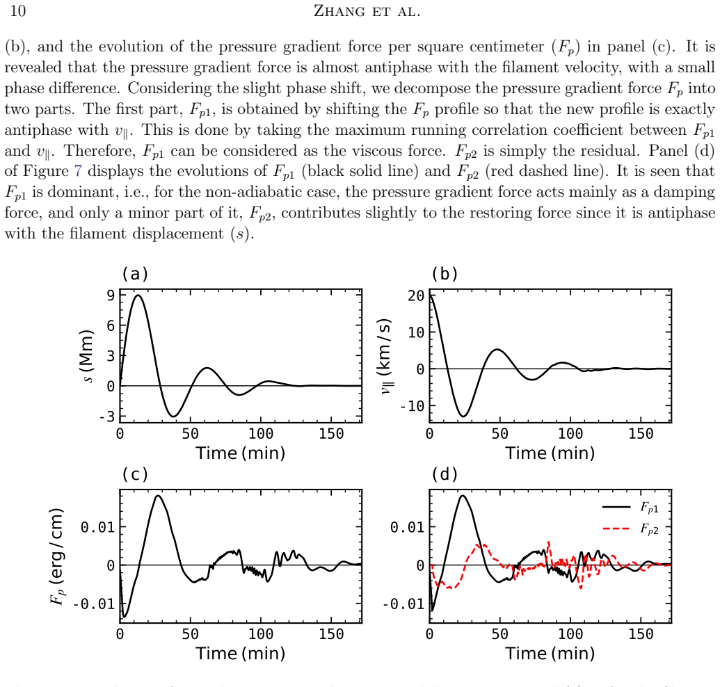
The load-bearing object is the dimensionless gravity-to-Lorentz ratio $\delta = \rho g L/(B^2/2\mu_0)$; when $\delta$ is near unity the dense filament can deform the magnetic field rather than sliding along a rigid tube. A second element is the pendulum relation $P=2\pi\sqrt{R/g}$, which the paper tests and finds wanting in that regime. The mechanism that carries the 2D damping is the piston effect: in a 2D slab the oscillating filament pushes all nearby field lines, generating transverse oscillations and outgoing fast-mode magnetoacoustic waves. The paper also decomposes the gas-pressure gradient force into a part antiphase with velocity (a viscous damping force in non-adiabatic runs) and a residual restoring part, explaining why radiation and heat conduction convert pressure forces from restoring to damping.
What would settle it
A 3D MHD simulation of a filament with $\delta\approx 1$ and a realistic sheared-core/unsheared-envelope field would settle it: if the decay time is not roughly half the matched 1D value and no fast-mode wave trains stream away from the filament, the wave-leakage claim fails. Observational support could come from detecting quasi-periodic 810 km/s wavefronts propagating above oscillating filaments in weak-field regions; their absence in many events would indicate the 2D piston picture does not apply.
Extended reading notes
Core claim
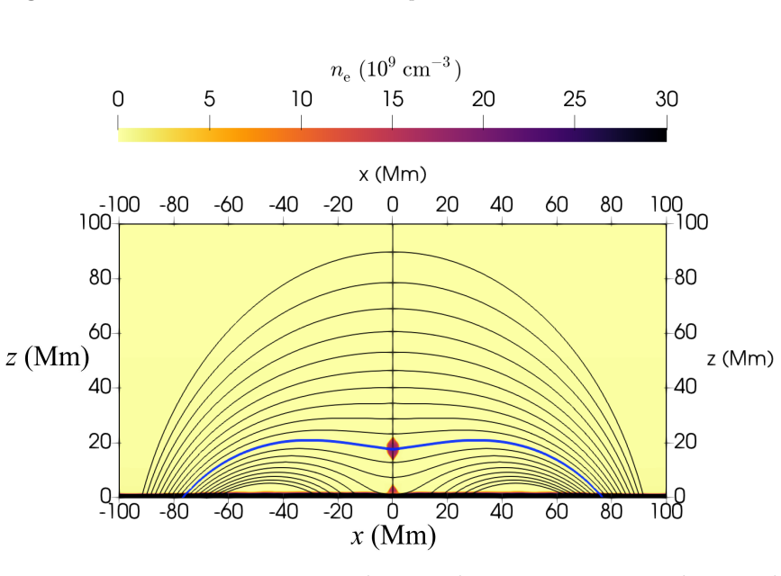
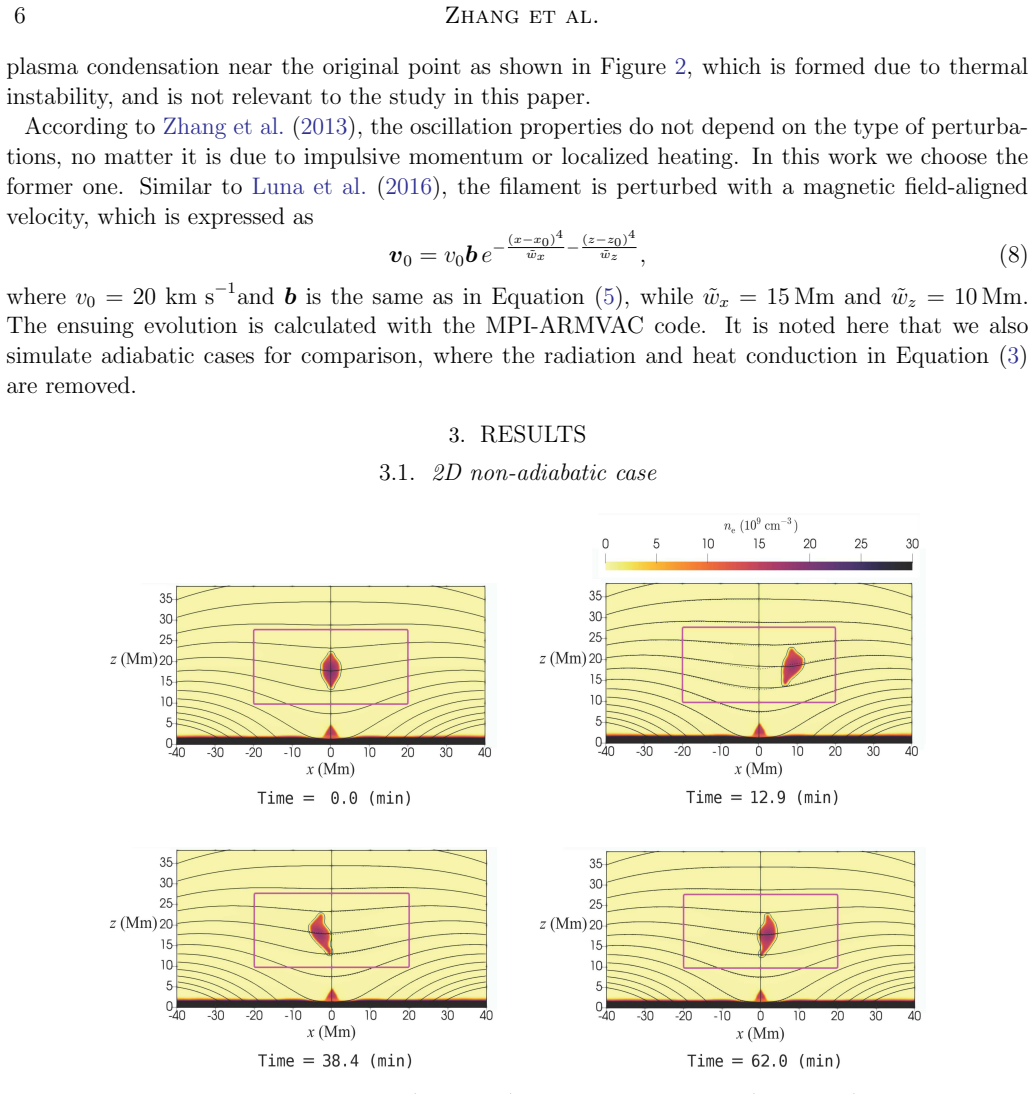
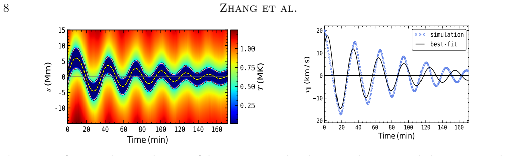
On its own terms, the paper reports that in a 2D non-adiabatic MHD simulation with the gravity-to-Lorentz ratio $\delta$ close to unity, a perturbed filament thread oscillates with period $P\approx 49$ minutes and decay time $\tau\approx 38$ minutes ($\tau \approx 0.7P$), whereas the matched 1D non-adiabatic run gives $P\approx 30$ minutes and $\tau\approx 76$ minutes ($\tau \approx 2.5P$). The 2D adiabatic run decays in about 211 minutes while the 1D adiabatic run is essentially decayless, isolating wave leakage as the extra 2D damping channel. The deformation of the field line by the moving filament excites a transverse oscillation with period $\approx 6.38$ minutes and quasi-periodic fast-mode waves that carry energy upward and downward at about 810 km/s; energy-budget integrals attribute the loss to Lorentz force and gas pressure work, i.e., to wave radiation. Because the field flattens as the filament moves and the period lengthens by over 50% relative to 1D, the pendulum model's inferred dip curvature radius is wrong by roughly 100% in this regime.
Load-bearing premise
The argument relies on the 2D slab result carrying over to the real three-dimensional Sun, where a filament's sheared core field is surrounded by a quasi-perpendicular envelope that forces the ambient field to oscillate like a piston; if the surrounding field lines are instead pushed aside, the extra damping and the 100% pendulum error would shrink substantially.
Editorial extensions
If this is right
- Observed decay times shorter than 1D predictions can be explained by wave leakage plus radiation and conduction, without needing mass drainage or thread-thread interaction.
- In weak-field events ($\delta\approx 1$), measured periods should not be fed directly into the pendulum formula; inferred dip curvature radii will be roughly twice too large.
- Longitudinal oscillations in this regime should be accompanied by small-amplitude transverse oscillations with periods of minutes and by upward and downward fast-mode wave trains in the surrounding corona.
- The predicted $\tau/P \approx 0.7$ is in line with the smallest observed damping ratios ($\approx 0.6$), suggesting wave leakage is a significant damping agent in real weak-field filaments.
- The transition between pendulum-valid and pendulum-invalid behavior is governed by $\delta$, not by plasma $\beta$; stronger-field filaments with $\delta\approx 0.2$ remain safe for the pendulum model.
Reading between the lines
- If the 2D piston picture survives in 3D for the sheared-core/unsheared-envelope geometry, then filament oscillations in weak-field regions should be observable sources of outward-propagating quasi-periodic coronal disturbances; a systematic search near oscillating filaments would test this.
- The period drift predicted here (the period shortens as the oscillation decays) could serve as an observational diagnostic of the $\delta$ regime even when the magnetic field strength is not directly measurable.
- The roughly 100% error bound is likely an upper limit for real filaments: in 3D geometries where ambient field lines slip sideways around the flux tube, wave leakage weakens and the pendulum model partially recovers.
- Energy carried away by leaked fast-mode waves is deposited in the ambient corona, so filament oscillations may contribute to local coronal heating near weak-field filaments, a consequence the paper does not quantify.
Signed reviews
Editorial analysis
A structured set of objections, weighed in public.
Referee Report
Summary. Zhang, Fang, and Chen present two-dimensional (2D) MHD simulations of a filament thread oscillating longitudinally in a dipped quadrupolar magnetic field with gravity-to-Lorentz force ratio δ close to unity. They compare 2D non-adiabatic, 2D adiabatic, 1D non-adiabatic, and 1D adiabatic runs, fitting the field-aligned velocity with a damped sine to extract period and decay time. The central findings are that non-adiabatic processes (radiation and heat conduction) reduce the decay time, that the 2D runs lose additional energy through outgoing fast-mode wave trains generated by magnetic-field deformation, and that in this regime the pendulum model may misestimate the curvature radius of the magnetic dip by about 100%.
Significance. If established, the paper would make two useful contributions: a quantitative demonstration that wave leakage can shorten filament longitudinal oscillation decay times when the magnetic field is weak, and a warning that the pendulum model used for prominence seismology may fail when gravity and Lorentz force are comparable. The strength of the paper is its concrete evidence for the wave-leakage channel: the time-distance diagram in Figure 11 shows quasi-periodic vertical-velocity disturbances propagating upward and downward at the coronal fast-mode speed, and the energy-budget decomposition in Figure 12 indicates that Lorentz-force and pressure work remove a major part of the initial kinetic energy. The δ parameter adopted from Zhou et al. (2018) gives a useful ordering scheme for when field deformation matters. However, the headline 100% curvature-radius error is not currently established, because it is based on a comparison that mixes thermal period shifts with magnetic deformation, and the paper contains several internal numerical inconsistencies in the reported periods and decay times.
major comments (3)
- [§4.3 and Abstract] The claim that the pendulum model leads to an error of ~100% in the curvature radius is not established by the comparison made in the text. The paper compares the 2D non-adiabatic period (P = 49 min) with the 1D non-adiabatic period (P = 30 min) and attributes the 19-minute difference to magnetic-field deformation. But the paper's own numbers show that switching on radiation and heat conduction shortens the 1D rigid-field period from 37 min (adiabatic) to 30 min, a 19% thermal shift, while the 2D adiabatic period is 44 min, only 19% longer than the 1D adiabatic period. A deformation-only comparison (2D adiabatic 44 min vs. 1D adiabatic 37 min) gives a period increase of about 19% and a curvature-radius error of about 40%, not 100%. In addition, the signals are chirped (the paper itself notes the period decreases with time), so the constant fitted periods depend on the fitting window and are quoted without uncertainties. A proper rigid-field adiabatic baseline, or a time-resolved period estimate, is needed before the abstract's '~100%' statement is used.
- [§3.2, §3.3, §4, and Summary] The decay times reported for the same cases are internally inconsistent. Section 3.2 gives τ = 76 min for the 1D non-adiabatic case, but Summary item (3) states the decay time is reduced from 113 min in 1D to 34 min in 2D. Section 3.2 gives τ = 38 min for the 2D non-adiabatic case, while the text in Section 4 and Summary items (2) and (3) use 34 min. Section 3.3 gives τ = 211 min for the 2D adiabatic case, but Section 4.2 states that the 2D adiabatic case has a decay time of 76 min. These are exactly the numbers used to quantify the factor-of-two reduction and the τ/P = 0.7 claim, so they must be reconciled and the quoted values corrected consistently throughout.
- [§4.2, final paragraph] The extrapolation from the 2D slab result to real 3D filaments is asserted rather than demonstrated. The paper argues that the filament's sheared core field overlain by an unsheared envelope means the oscillating filament acts as a piston even in 3D, so wave leakage remains efficient. However, no 3D simulation or quantitative estimate of the piston efficiency is provided, and the paper itself notes that Terradas et al. (2006) found wave leakage ineffective for 3D flux tubes in an aligned ambient field. If, in 3D, the ambient field lines are pushed aside rather than forced to oscillate, the wave-leakage channel and the associated seismology error could be substantially smaller. Because the abstract's general claim about real filaments depends on this extrapolation, the paper should either add a 3D test, provide a quantitative geometric estimate, or explicitly restrict the claim to the 2D slab configuration.
minor comments (5)
- [Summary, item (1)] There is a typo: 'tha application of the pendulum model' should read 'the application of the pendulum model.'
- [§4.1, Figure 7 discussion] The text refers to 'shifting Tp' in the decomposition of the pressure-gradient force, but the variable is Fp throughout the section; this should be corrected.
- [Figure 4 caption] The caption contains 'Time-distance diagram of of the temperature distribution'; the duplicate 'of' should be removed.
- [§3.1 and §3.2] The damped-sine fits are described as reasonable for only the first 1.5 periods, with deviations becoming remarkable afterward, yet the extracted periods and decay times are quoted without uncertainties or a goodness-of-fit measure; reporting the fitting window and uncertainties would make the quantitative comparisons more robust.
- [§2, boundary conditions] The two side boundaries are reflecting; a brief discussion of whether waves reflected from these boundaries affect the measured decay times would help the reader assess the numerical setup.
Circularity Check
No circularity: the wave-leakage result is independently produced by the MHD simulations; self-citations are contextual and not load-bearing.
full rationale
The central wave-leakage result is an output of solving the stated MHD equations (Eqs. 1-5), with initial conditions taken from a quadrupolar field and a dense thread; no parameter is fitted to force the conclusion. The damped-sine fit (Eq. 9) is a post-processing characterization of the simulated centroid velocity, so the reported period and decay-time values describe outputs rather than acting as inputs. The 2D-vs-1D decay-time reduction is read directly from the four simulation runs, and the wave-leakage interpretation is independently supported by the energy-budget integrals (Fig. 12), the outgoing fast-mode wave trains (Fig. 11), and the induced transverse oscillation (Fig. 10). The delta parameter is taken from the same group's earlier paper (Zhou et al. 2018), but it is a dimensionless force ratio used to choose the regime; the new simulation verifies the expected behavior rather than importing it. Citations to Zhang et al. (2012, 2013) supply background and 1D baselines, but they do not by themselves produce the 2D results. The headline ~100% pendulum-error estimate does raise a correctness concern, not a circularity one: it is computed by comparing the 1D non-adiabatic period (30 min) with the 2D non-adiabatic period (49 min), although the 1D adiabatic period is 37 min and the 2D adiabatic period is 44 min, so the comparison appears to mix thermal period shortening with field-deformation lengthening. This weakens the quantitative claim but does not make the derivation circular.
Assumptions & free parameters
free parameters (6)
- B0 = 10 G (quadrupolar field amplitude) =
10 G
- Quadrupolar field wavenumbers k1 and k2 =
k1=pi/200 Mm^-1, k2=3 k1
- Filament density contrast delta_rho/rho_corona =
99
- Initial perturbation amplitude v0 =
20 km/s
- Background heating amplitude H0 and scale height Hm =
H0=1.5e-4 erg/cm^3/s, Hm=40 Mm
- Thread dimensions wx and wz =
wx=4 Mm, wz=3 Mm
assumptions (6)
- domain assumption Ideal MHD with field-aligned Spitzer heat conduction and optically thin radiative loss describes the filament-corona system.
- domain assumption The relaxed atmosphere reached after 110 minutes, then after inserting the filament and re-running, is a valid initial equilibrium for the oscillation study.
- domain assumption The standard pendulum relation between period and dip curvature radius is the accepted baseline for filament seismology.
- ad hoc to paper The pressure-gradient force decomposition using the maximum running correlation between Fp and velocity or displacement separates restoring from damping components.
- ad hoc to paper The 2D slab result that wave leakage is efficient carries over to 3D because the filament's envelope field is quasi-perpendicular to the core field, so the oscillating filament acts as a piston in 3D.
- domain assumption The dimensionless parameter delta = rho g L / (B^2 / 2 mu0) governs whether the filament gravity deforms the magnetic field.
Cite this review
Pith. "Pith review of Damping Mechanisms of the Solar Filament Longitudinal Oscillations in Weak Magnetic Field." pith.science (2026). https://pith.science/paper/SGN5EPB2
@misc{pith2026190807148,
  author       = {Pith},
  title        = {Pith review of: Damping Mechanisms of the Solar Filament Longitudinal Oscillations in Weak Magnetic Field},
  year         = {2026},
  howpublished = {\url{https://pith.science/paper/SGN5EPB2}},
  note         = {Machine review of arXiv:1908.07148}
}
read the original abstract
Longitudinal oscillations of solar filament have been investigated via numerical simulations continuously, but mainly in one dimension (1D), where the magnetic field line is treated as a rigid flux tube. Whereas those one-dimensional simulations can roughly reproduce the observed oscillation periods, implying that gravity is the main restoring force for filament longitudinal oscillations, the decay time in one-dimensional simulations is generally longer than in observations. In this paper, we perform a two-dimensional (2D) non-adiabatic magnetohydrodynamic simulation of filament longitudinal oscillations, and compare it with the 2D adiabatic case and 1D adiabatic and non-adiabatic cases. It is found that, whereas both non-adiabatic processes (radiation and heat conduction) can significantly reduce the decay time, wave leakage is another important mechanism to dissipate the kinetic energy of the oscillating filament when the magnetic field is weak so that gravity is comparable to Lorentz force. In this case, our simulations indicate that the pendulum model might lead to an error of ~100% in determining the curvature radius of the dipped magnetic field using the longitudinal oscillation period when the gravity to Lorentz force ratio is close to unity.
Figures

Figures from the paper (9 more)



Reference graph
Works this paper leans on
-
[1]
Arregui, I., Oliver, R., & Ballester, J. L. 2018, Living Reviews in Solar Physics, 15, 3, doi: 10.1007/s41116-018-0012-6
-
[2]
Brady, C. S., & Arber, T. D. 2005, A&A, 438, 733, doi: 10.1051/0004-6361:20042527
-
[3]
Cally, P. S. 1986, SoPh, 103, 277, doi: 10.1007/BF00147830 Damping of filament longitudinal oscillations 17
-
[4]
Chen, P. F. 2011, Living Reviews in Solar Physics, 8, 1, doi: 10.12942/lrsp-2011-1
-
[5]
Chen, P. F., Harra, L. K., & Fang, C. 2014, ApJ, 784, 50, doi: 10.1088/0004-637X/784/1/50 D´ ıaz, A. J., Zaqarashvili, T., & Roberts, B. 2006, A&A, 455, 709, doi: 10.1051/0004-6361:20054430
-
[6]
Hillier, A., Morton, R. J., & Erd´ elyi, R. 2013, ApJL, 779, L16, doi: 10.1088/2041-8205/779/2/L16
-
[7]
Jing, J., Lee, J., Spirock, T. J., et al. 2003, ApJ, 584, L103, doi: 10.1086/373886
doi:10.1086/373886 2003
-
[8]
Klimchuk, J. A., & MacNeice, P. J. 2001, ApJL, 553, L85, doi: 10.1086/320497
Show all 34 references
-
[9]
2012, Journal of Computational Physics, 231, 718, doi: 10.1016/j.jcp.2011.01.020
Keppens, R., Meliani, Z., van Marle, A., et al. 2012, Journal of Computational Physics, 231, 718, doi: 10.1016/j.jcp.2011.01.020
2012 doi
-
[10]
1957, ZA, 43, 36
Kippenhahn, R., & Schl¨ uter, A. 1957, ZA, 43, 36
1957
-
[11]
Kuperus, M., & Raadu, M. A. 1974, A&A, 31, 189
1974
-
[12]
2012, ApJL, 760, L10, doi: 10.1088/2041-8205/760/1/L10
Li, T., & Zhang, J. 2012, ApJL, 760, L10, doi: 10.1088/2041-8205/760/1/L10
2012 doi
-
[13]
R., & Wiik, J
Lin, Y., Engvold, O. R., & Wiik, J. E. 2003, SoPh, 216, 109, doi: 10.1023/A:1026150809598
2003 doi
-
[14]
V., et al
Liu, W., Ofman, L., Nitta, N. V., et al. 2012, ApJ, 753, 52, doi: 10.1088/0004-637X/753/1/52
2012 doi
-
[15]
L., et al
Luna, M., Karpen, J., Ballester, J. L., et al. 2018, ApJS, 236, 35, doi: 10.3847/1538-4365/aabde7
2018 doi
-
[16]
Luna, M., & Karpen, J. T. 2012, ApJ, 750, L1, doi: 10.1088/2041-8205/750/1/L1
2012 doi
-
[17]
2016, ApJ, 817, 157, doi: 10.3847/0004-637X/817/2/157
Luna, M., Terradas, J., Khomenko, E., Collados, M., & de Vicente, A. 2016, ApJ, 817, 157, doi: 10.3847/0004-637X/817/2/157
2016 doi
-
[18]
2014, Living Reviews in Solar Physics, 11, 1, doi: 10.12942/lrsp-2014-1
Parenti, S. 2014, Living Reviews in Solar Physics, 11, 1, doi: 10.12942/lrsp-2014-1
2014 doi
-
[19]
2014, The Astrophysical Journal Supplement Series, 214, 4, doi: 10.1088/0067-0049/214/1/4
Keppens, R. 2014, The Astrophysical Journal Supplement Series, 214, 4, doi: 10.1088/0067-0049/214/1/4
2014 doi
-
[20]
2009, A&A, 508, 751, doi: 10.1051/0004-6361/200912495
Keppens, R., & Vink, J. 2009, A&A, 508, 751, doi: 10.1051/0004-6361/200912495
2009 doi
-
[21]
K., Murawski, K., Wang, T
Selwa, M., Solanki, S. K., Murawski, K., Wang, T. J., & Shumlak, U. 2006, A&A, 454, 653, doi: 10.1051/0004-6361:20054286
2006 doi
-
[22]
D., Chen, P
Shen, Y., Liu, Y. D., Chen, P. F., & Ichimoto, K. 2014, ApJ, 795, 130, doi: 10.1088/0004-637X/795/2/130
2014 doi
-
[23]
Terradas, J., Oliver, R., & Ballester, J. L. 2006, ApJL, 650, L91, doi: 10.1086/508569
2006 doi
-
[24]
2009, SSRv, 149, 283, doi: 10.1007/s11214-009-9583-9
Tripathi, D., Isobe, H., & Jain, R. 2009, SSRv, 149, 283, doi: 10.1007/s11214-009-9583-9
2009 doi
-
[25]
Verwichte, E., Foullon, C., & Nakariakov, V. M. 2006, A&A, 452, 615, doi: 10.1051/0004-6361:20054437 Vrˇ snak, B., Veronig, A. M., Thalmann, J. K., & ˇZic, T. 2007, A&A, 471, 295, doi: 10.1051/0004-6361:20077668
2006 doi
-
[26]
1999, ApJL, 520, L71, doi: 10.1086/312149
Wang, Y.-M. 1999, ApJL, 520, L71, doi: 10.1086/312149
1999 doi
-
[27]
2018, The Astrophysical Journal Supplement Series, 234, 30, doi: 10.3847/1538-4365/aaa6c8
Keppens, R. 2018, The Astrophysical Journal Supplement Series, 234, 30, doi: 10.3847/1538-4365/aaa6c8
2018 doi
-
[28]
M., Chen, P
Zhang, Q. M., Chen, P. F., Xia, C., & Keppens, R. 2012, A&A, 542, A52, doi: 10.1051/0004-6361/201218786
2012 doi
-
[29]
M., Chen, P
Zhang, Q. M., Chen, P. F., Xia, C., Keppens, R., & Ji, H. S. 2013, A&A, 554, A124, doi: 10.1051/0004-6361/201220705
2013 doi
-
[30]
M., Li, D., & Ning, Z
Zhang, Q. M., Li, D., & Ning, Z. J. 2017, ApJ, 851, 47, doi: 10.3847/1538-4357/aa9898
2017 doi
-
[31]
Chen, P. F. 2018, ApJ, 856, 179, doi: 10.3847/1538-4357/aab614
2018 doi
-
[32]
B., Engvold, O., & Martin, S
Zirker, J. B., Engvold, O., & Martin, S. F. 1998, Nature, 396, 440, doi: 10.1038/24798
1998 doi
-
[33]
F., Yang, K., & Cao, W
Zou, P., Fang, C., Chen, P. F., Yang, K., & Cao, W. 2017, ApJ, 836, 122, doi: 10.3847/1538-4357/836/1/122
2017 doi
-
[34]
F., et al
Zou, P., Fang, C., Chen, P. F., et al. 2016, ApJ, 831, 123, doi: 10.3847/0004-637X/831/2/123
2016 doi
Reviewed August 14, 2026 · model on record in the stance chip above.
Discussion (0). Continue with ORCID to comment.