REVIEW 2 major objections 5 minor 9 references
Improvements to Warm-Started Optimized Trajectory Planning for ASVs
T0 review · 2 major / 5 minor · reviewed 2026-08-14 · deepseek-v4-flash
Pith's one-line read Replacing the uniform grid with a Voronoi diagram cuts the first two stages of an ASV trajectory planner from 5.6 s to 0.8 s while keeping the energy cost nearly identical.
desk verdict Real 85% Step 1–2 speedup on the tested scenario, but the coarsely sampled Voronoi graph's completeness is asserted rather than shown; deserves review with requests for more scenarios and repeated trials. read the letter →
The pith
A machine-rendered reading of the paper's core claim, the machinery that carries it, and where it could break.
The reading
What carries the argument
The load-bearing object is the Voronoi diagram of the obstacle map, built from generator points spaced at $\Delta d = 100$ m along obstacle boundaries and map edges. A Voronoi diagram partitions the map into cells around generators so that every point in a cell is closer to its own generator than to any other, and the cell boundaries form a searchable graph whose nodes are pushed as far from obstacles as possible. The paper's key structural fact is that this graph retains a route between every pair of obstacles even at coarse spacing, unlike a uniform grid of comparable node count. A* runs on this sparse graph to find the shortest piecewise-linear path, and the cited refinement scheme iteratively cuts corners of adjacent edges to shorten the Voronoi path while preserving collision-free clearance. The remaining machinery is the warm-start generation for the nonlinear program: circle arcs smooth the path, artificial temporal information makes it a trajectory, and improved Euler integration propagates the cost-to-go (instead of Runge-Kutta 4) to produce an initial guess for the optimal control solver.
What would settle it
Run the same two planners on a map whose only viable route passes through a corridor narrower than the Voronoi generator spacing and whose obstacle layout makes the Voronoi edge bypass that corridor; if the Voronoi-based A* returns a visibly longer path or the final energy cost rises well above the dense-grid result, the 'same optimality' claim fails in that setting.
Extended reading notes
Core claim
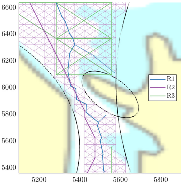
The central claim is that the two slow front-end stages of the warm-started trajectory planner can be accelerated by replacing the uniform map grid with a Voronoi diagram built from obstacle-boundary generator points. The Voronoi graph is far sparser than the dense 50 m grid (833 non-colliding nodes versus 22,929), yet it still contains paths between all obstacles, so the A* search finds the same shortest piecewise-linear route through the map's narrow central passage that the dense grid finds. Because Voronoi edges sit far from obstacle boundaries, the extracted path is longer, so the authors append the path-refinement and waypoint-reduction scheme from a cited earlier work to pull the path closer to obstacles, and they replace Runge-Kutta 4 integration with improved Euler integration when generating the optimal control warm start. On the test scenario, Step 1 falls from 3.4 s to 0.7 s and Step 2 from 2.2 s to 0.1 s, for an 85% reduction in the combined run time of the first two steps, while the final energy-optimal trajectories agree closely: $2.75\cdot10^{7}$ J for the improved method versus $2.74\cdot10^{7}$ J for the original dense-grid method. The authors additionally claim completeness of the global search in the sense that the Voronoi graph keeps routes between all obstacles even at coarse generator spacing, whereas an equally sparse uniform grid (843 nodes at 270 m spacing) loses the central passage and produces a $3.85\cdot10^{7}$ J trajectory.
Load-bearing premise
The load-bearing premise is that a Voronoi diagram built from obstacle-boundary generators spaced 100 m apart keeps every route that matters, including the narrow central passage, in its search space even when a uniform grid at comparable spacing would lose that passage.
Editorial extensions
If this is right
- The combined front-end run time drops from about 5.6 s to 0.8 s in the test scenario, so the global search can be re-run far more often during an ASV mission.
- The sparse Voronoi grid reaches essentially the same final energy-optimal trajectory as the dense 50 m uniform grid ($2.75\cdot10^{7}$ J versus $2.74\cdot10^{7}$ J), so this speedup does not visibly trade away trajectory quality in the demonstrated case.
- An equally sparse uniform grid (843 nodes) does not preserve quality: it misses the narrow central passage and produces a $3.85\cdot10^{7}$ J trajectory, showing that node count alone cannot replace connectivity-preserving structure.
- The optimal control step still dominates total run time (16.6 s of 17.4 s), so the headline 85% figure describes the front-end stages, not the whole pipeline.
Reading between the lines
- The same substitution should transfer to other roadmap-plus-optimization planners: whenever narrow corridors matter, a connectivity-preserving sparse graph can deliver the speed of coarse sampling without the route loss of a coarse uniform grid.
- The size of the gain is scenario-dependent; a practical design rule would tie the Voronoi generator spacing $\Delta d$ to the narrowest corridor the vehicle must be able to traverse.
- Because Step 3 accounts for most of the run time, the practical payoff of these front-end improvements is more frequent global re-planning, not a proportionally faster final trajectory.
- Using improved Euler instead of Runge-Kutta 4 in Step 2 is safe only because Step 2 produces an initial guess; the same accuracy trade-off would need separate validation inside the final optimal control solve.
Signed reviews
Editorial analysis
A structured set of objections, weighed in public.
Referee Report
Summary. Bitar et al. present three modifications to the warm-started pipelined trajectory planner of Bitar et al. (2019) for autonomous surface vehicles: (i) replacing the uniform grid used by the A* search with a Voronoi diagram whose generators are obstacle-boundary samples spaced by Δd = 100 m; (ii) applying the path-refinement and waypoint-reduction scheme of Bhattacharya and Gavrilova (2008) in Step 2; and (iii) swapping Runge-Kutta 4 integration for improved Euler integration in the warm-start construction. On a single island scenario, three configurations are compared: R1 (Voronoi, 833 nodes), R2 (original dense uniform grid, 22,929 nodes), and R3 (coarse uniform grid, 843 nodes). Table 2 reports that R1 and R2 achieve nearly equal energy cost (2.75 vs 2.74 × 10^7 J) while Step 1 time drops from 3.4 s to 0.7 s and Step 2 from 2.2 s to 0.1 s, an 85% reduction in Steps 1+2 time. R3 misses the narrow central passage because of grid disconnection and yields a 3.85 × 10^7 J trajectory. The paper concludes that the Voronoi discretization 'keeps paths between all obstacles ... even when they are coarsely discretized,' and hence that the method remains complete in terms of the shortest path.
Significance. If the claimed speedup and comparable optimality are robust, the paper offers a practically useful reduction in the warm-starting cost of a dynamic trajectory planner, and the Voronoi-based sparse search graph is a sensible alternative to a dense uniform grid. The paper has concrete strengths: the comparison with R3 is a well-chosen control that isolates the effect of the sparse search structure; the arithmetic behind the 85% figure is consistent with Table 2 (1 − 0.8/5.6 ≈ 0.857); the cost function, model, and solver are inherited from prior work rather than tuned to the reported result; and the improvement in Steps 1 and 2 is clearly quantified. The main weakness is that the general completeness/optimality claim is asserted rather than demonstrated outside the single example, and all timings are single runs. The result is significant for the specific scenario; its broader significance depends on whether the Voronoi completeness assertion can be substantiated or appropriately qualified.
major comments (2)
- [Section 5 (completeness claim) and Section 3 (Voronoi construction)] The conclusion asserts that 'The Voronoi diagram keeps paths between all obstacles in the search space even when they are coarsely discretized' and that the method is 'complete in terms of the shortest path.' This is the load-bearing premise for the claim that the 85% Step 1-2 reduction maintains optimality. The graph used here, however, is not the continuous generalized Voronoi diagram of the obstacles but the Voronoi diagram of boundary samples spaced at Δd = 100 m (Section 3, R1 in Section 4). Coarse sampling can omit narrow free-space passages, exactly as the R3 uniform grid with 843 nodes omits the central passage on this map (Section 4, Figures 3-4). No stress test or argument is provided to show that the Δd = 100 m Voronoi sample retains the true shortest route on other maps or spacings. Since Step 3 is a local OCP warm-started by the Step 1-2 path, a passage absent after Step 1 cannot be recovered later. Please either prove or disprove the completeness property under boundary sampling, provide a counterexample analysis, or restrict the optimality claim to the demonstrated scenario.
- [Section 4, Table 2] The 85% speedup and the 'virtually equal energy' comparison rest on single measurements: Table 2 reports one run time and one energy value per configuration, with no repeated trials, variance, or machine/implementation details. A* and Ipopt are deterministic in iteration counts but wall-clock times are environmental, and the energy difference between R1 and R2 (2.75 vs 2.74 × 10^7 J) is 0.36% with no tolerance stated for what 'same level of optimality' means. Please report multiple runs (at least for the runtime comparison), or state explicitly that the times are single runs and treat the 85% figure as an illustration rather than a measured performance guarantee.
minor comments (5)
- [Abstract and Section 5] The phrase 'the first part of the method' is ambiguous: the 85% reduction refers to Steps 1 and 2 combined, not to Step 1 alone or to the entire pipeline. Consider saying 'Steps 1 and 2' explicitly, since Table 2 shows that Step 3 still dominates the total runtime (16.6 of 17.4 s for R1).
- [Section 4, paragraph 2] The sentence 'We see that the Voronoi diagram proposes all possible routes between the obstacles as paths' is stronger than what a single map can show; suggest changing to 'all possible routes in this scenario' or adding a proof/reference for the general claim.
- [Section 2.1 and Table 1] The statement that a Voronoi discretization 'can contain all possible paths between obstacles, while the map is sparsely discretized' is presented as an established property before the evidence in Section 4. It should be flagged as an assumption or supported by a citation that specifically covers coarse boundary sampling, not just the continuous Voronoi diagram.
- [Section 3] The path-refinement and waypoint-reduction steps are described only verbally as 'iteratively cutting corners of two edges' and via a reference to Bhattacharya and Gavrilova (2008). A pseudocode block or a precise algorithmic description would materially improve reproducibility.
- [Section 4, R3 definition] R3 is described as having 'the same number of nodes' as R1 in the text, but the table in Section 4 gives 843 vs 833 nodes; using 'comparable number of nodes' would be more accurate.
Circularity Check
No significant circularity: the runtime reduction is an empirical comparison against the authors' own baseline, with no fitted parameter renamed as a prediction.
full rationale
The paper's central quantitative claim is an empirical runtime comparison: Step 1 drops from 3.4 s to 0.7 s, Step 2 from 2.2 s to 0.1 s, with final energy costs of 2.74e7 J and 2.75e7 J (Table 2). These are measurements against the authors' prior method (Bitar et al. 2019), used appropriately as a baseline; no parameter is fitted to the reported outcome and no fitted quantity is relabeled as a prediction. The Voronoi replacement is justified by a standard geometric property of Voronoi diagrams, and the paper's completeness claim ('The Voronoi diagram keeps paths between all obstacles in the search space even when they are coarsely discretized') is a testable assumption, not a restatement of the result. The R3 control demonstrates that a sparse uniform grid misses the narrow passage, while R1 and R2 both find it in the example, which supports the 'same optimality' claim for this scenario. Any concern that the completeness claim may fail for other maps or spacings is a correctness or generalization risk, not circularity. The self-citations to Bitar et al. 2019 and Bhattacharya and Gavrilova are contextual baselines or independent external sources, and no load-bearing uniqueness theorem is imported from the authors. Therefore no circular step is exhibited.
Assumptions & free parameters
free parameters (2)
- Voronoi generator spacing delta_d =
100 m
- Cost weights K_e and K_t =
Inherited from Bitar et al. 2019; not restated numerically in this paper
assumptions (4)
- domain assumption A Voronoi diagram built from generators along obstacle boundaries contains all possible collision-free routes between obstacles.
- domain assumption The shortcutting refinement from Bhattacharya and Gavrilova preserves collision avoidance while shortening the path.
- domain assumption After Voronoi-based warm starting, the NLP solver finds a local optimum comparable to the dense-grid warm start.
- domain assumption The ASV model and OCP transcription from Bitar et al. 2019 are accepted as correct.
Cite this review
Pith. "Pith review of Improvements to Warm-Started Optimized Trajectory Planning for ASVs." pith.science (2026). https://pith.science/paper/LP75ZSGX
@misc{pith2026190807311,
  author       = {Pith},
  title        = {Pith review of: Improvements to Warm-Started Optimized Trajectory Planning for ASVs},
  year         = {2026},
  howpublished = {\url{https://pith.science/paper/LP75ZSGX}},
  note         = {Machine review of arXiv:1908.07311}
}
read the original abstract
We present improvements to a recently developed method for trajectory planning for autonomous surface vehicles (ASVs) in terms of run time. The original method combines two types of planners: An A* implementation that quickly finds the global shortest piecewise linear path on a uniformly discretized map, and an optimal control-based trajectory planner which takes into account ASV dynamics. Firstly, we propose an improvement to the discretization of the map by switching to a Voronoi diagram rather than the uniform discretization, which offers a far more sparse search tree for the A* implementation. Secondly, modifications to the path refinement are made, as suggested in a paper by Bhattacharya and Gavrilova. The changes result in a reduction to the run time of the first part of the method of 85% for an example scenario while maintaining the same level of optimality.
Figures


Figures from the paper (3 more)


Reference graph
Works this paper leans on
-
[1]
CasADi – A software framework for nonlinear optimization and optimal control
Andersson, J. A. E., J. Gillis, G. Horn, J. B. Rawlings, and M. Diehl (2018). “CasADi – A software framework for nonlinear optimization and optimal control”. In: Mathematical Programming Compu- tation
work page 2018
-
[2]
Voronoi Diagrams – A Survey of a Fundamental Geometric Data Structure
Aurenhammer, F. (1991). “Voronoi Diagrams – A Survey of a Fundamental Geometric Data Structure”. In: ACM Computing Surveys 23.3, pp. 345–405
work page 1991
-
[3]
Roadmap-Based Path Planning - Using the Voronoi Diagram for a Clearance-Based Shortest Path
Bhattacharya, P. and M. Gavrilova (2008). “Roadmap-Based Path Planning - Using the Voronoi Diagram for a Clearance-Based Shortest Path”. In: IEEE Robotics & Automation Magazine 15.2, pp. 58–66
work page 2008
-
[4]
Warm-Started Optimized Trajectory Planning for ASVs
Bitar, G., V. N. Vestad, A. M. Lekkas, and M. Breivik (2019). Warm-Started Optimized Trajectory Plan- ning for ASVs . Accepted to the 12th IFAC Conference on Control Applications in Marine Systems, Robotics, and Vehicles. arXiv: 1907.02696 [eess.SY]. Bortoff, S. A. (2000). “Path planning for UAVs”. In:Proceedings of the ’00 American Control Conference
work page Pith review arXiv 2019
-
[5]
A Voronoi-diagram-based dynamic path- planning system for underactuated marine vessels
Candeloro, M., A. M. Lekkas, and A. J. Sørensen (2017). “A Voronoi-diagram-based dynamic path- planning system for underactuated marine vessels”. In: Control Engineering Practice 61, pp. 41–54
work page 2017
-
[6]
MPC-based Mid-level Collision Avoidance for ASVs using Nonlinear Programming
Eriksen, B.-O. H. and M. Breivik (2017). “MPC-based Mid-level Collision Avoidance for ASVs using Nonlinear Programming”. In: Proceedings of the 2017 IEEE Conference on Control Technology and Applications (CCTA). Mauna Lani, HI, USA, pp. 766–772
work page 2017
-
[7]
Tessellations in GIS: Part II–making changes
Gold, C. (2016). “Tessellations in GIS: Part II–making changes”. In: Geo-spatial Information Science 19.2, pp. 157–167
work page 2016
-
[8]
A formal basis for the heuristic determination of minimum cost paths
Hart, P., N. Nilsson, and B. Raphael (1968). “A formal basis for the heuristic determination of minimum cost paths”. In: IEEE Transactions on Systems Science and Cybernetics 4.2, pp. 100–107
work page 1968
Show all 9 references
-
[9]
Bering Sea ASV Force Multiplier
Orthmann, A. (2016). “Bering Sea ASV Force Multiplier”. In: Hydro International. url: https://www. hydro- international.com/content/article/bering- sea- asv- force- multiplier (visited on 2019-08-16). W¨ achter, A. and L. T. Biegler (2005). “On the implementation of an interio...
2016
Reviewed August 14, 2026 · model on record in the stance chip above.
Discussion (0). Continue with ORCID to comment.