Stochastic differential theory of cricket

Santosh Kumar Radha

REVIEW 5 major objections 5 minor 17 references

Stochastic differential theory of cricket

T0 review · 5 major / 5 minor · reviewed 2026-08-14 · deepseek-v4-flash

Challenge this review Re-run · record.json Download PDF Read on arXiv ↗ Review JSON

Pith's one-line read This paper argues that a cricket match's progression is captured by one mean-reverting stochastic variable, so that every team is characterized by three parameters and the win probability can be updated ball by ball.

desk verdict A cricket-specific SDE state variable with real analytic potential, but the published formulas—especially Equation 15—contradict the model they are derived from, so the central claim is unsupported as written. read the letter →

arxiv 1908.07372 v1 pith:7ZKGMX66 submitted 2019-08-12 physics.soc-ph math.PRstat.APstat.OT

Santosh Kumar Radha This is my paper · ORCID

classification physics.soc-phmath.PRstat.APstat.OT MSC 60H1060J70

keywords stochasticdifferentialequationOrnstein-Uhlenbeckprocesscricketwinprobabilitysportsanalyticsnetrunratemeanreversion

verification ladder T0 review T1 audit T2 compute T3 formal

The pith

A machine-rendered reading of the paper's core claim, the machinery that carries it, and where it could break.

The reading

This paper introduces a stochastic differential equation formalism for cricket, centered on the lead variable $X_t = NR(t) - RR(t)$, the difference between net run rate per ball and required run rate per ball. It argues that $X_t$ evolves as an Ornstein-Uhlenbeck process $dX_t = x_0(x_1 - X_t)dt + \sigma dW_t$, which makes the final lead conditionally Gaussian and gives a closed-form win probability at any ball. If correct, every team reduces to three physically meaningful numbers—reversion speed, long-run average lead, and volatility—and live win probabilities can be computed from the current match state. The paper demonstrates the approach on a real India–Sri Lanka match, where the probability stays near 0.5 even when the raw lead looks negative.

What carries the argument

The load-bearing object is the Ornstein-Uhlenbeck process in Eq. (11), a mean-reverting random walk with constant volatility. Its explicit solution is Gaussian, so the conditional distribution of the final lead given the current lead is normal with mean $\alpha e^{-x_0(1-t)} + x_1(1 - e^{-x_0(1-t)})$ and the corresponding variance; Eq. (15) is the tail probability of that normal above zero. The same equations yield the stationary mean $x_1$ and stationary variance $\sigma^2/(2x_0)$, which is how the physical meanings of the three parameters are extracted.

What would settle it

Take a large sample of real matches and, for many time points $t$ and observed leads $\alpha$, compare the empirical frequency of wins with Eq. (15) evaluated at the fitted $(x_0, x_1, \sigma)$. If the residuals $X(1) - E[X(1) \mid X(t)=\alpha]$ are skewed or heavy-tailed, or if the fitted parameters drift systematically across opponents, the central claim is falsified.

Watch

Extended reading notes

Core claim

The central claim is that the net-run-rate lead is the fundamental state variable of a cricket match, not a heuristic scoreboard statistic. Its evolution is $dX_t = x_0(x_1 - X_t)dt + \sigma dW_t$, an Ornstein-Uhlenbeck process whose solution yields closed-form expressions for the mean, $E[X_t]$, and variance, $Var[X_t]$. The probability that the second-innings team wins at the end, $P(X(1)>0 \mid X(t)=\alpha)$, is then the explicit error-function expression in Eq. (15). The three fitted constants receive physical interpretations: $x_1$ is the long-run lead the team tends to settle at, $x_0$ controls how quickly it returns there, and $\sigma$ measures unpredictability.

Load-bearing premise

The whole calculation rests on assuming that $X_t$ follows the Ornstein-Uhlenbeck process $dX_t = x_0(x_1 - X_t)dt + \sigma dW_t$ with constant, historically fitted parameters, so that the final lead is conditionally normal with the mean and variance from Eqs. 13–14; if real match dynamics are not mean-reverting with constant volatility, Eq. 15 is not the true win probability.

Editorial extensions

If this is right

A team's quality is summarized by the vector $(x_0, x_1, \sigma)$, so head-to-head comparisons reduce to comparing these three numbers instead of combining arbitrary rating statistics.
Given any ball index $t$ and current lead $\alpha$, Eq. (15) gives an explicit update of the chasing team's win probability, allowing live odds to be refreshed ball by ball.
The long-run mean $x_1$ and stationary variance $\sigma^2/(2x_0)$ separate 'how good a team is' from 'how unpredictable a team is'.
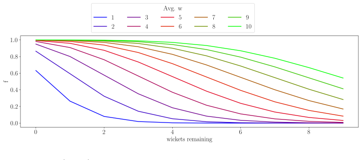
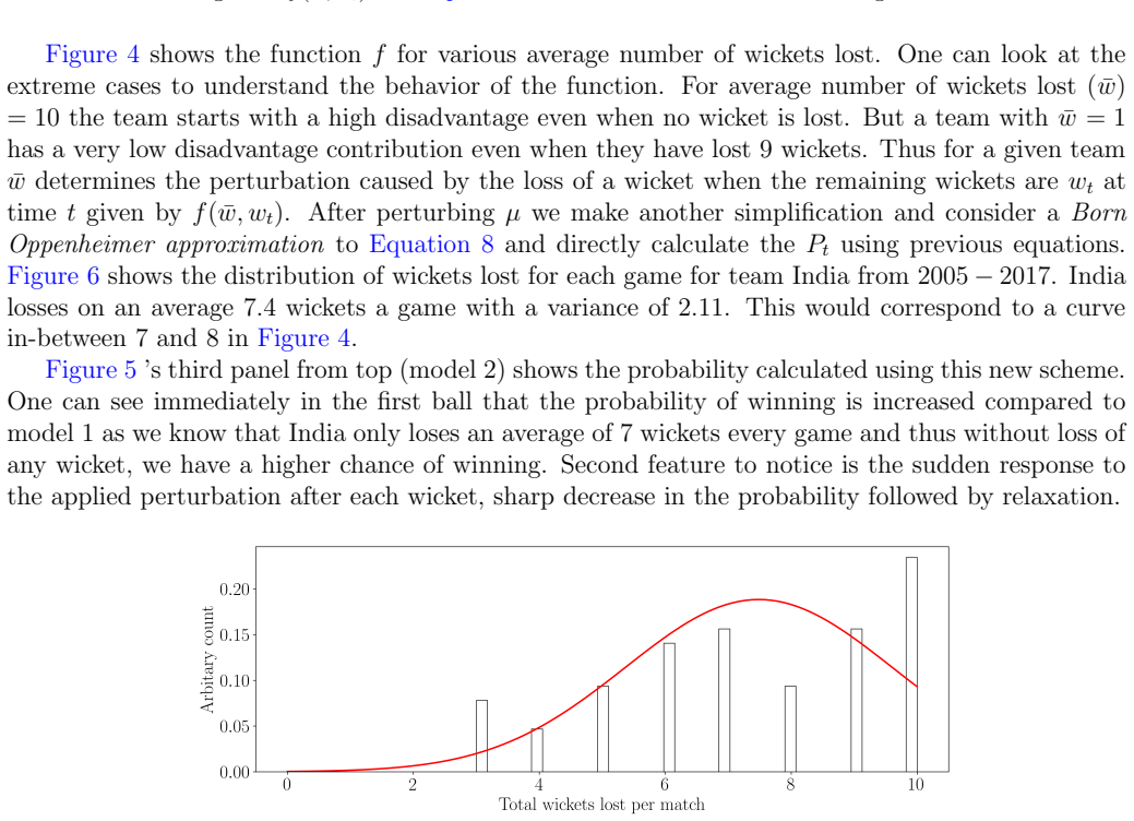
Fitting Eqs. (13)–(14) to historical ball-by-ball data recovers the observed mean and variance trajectories, and Model 2 shows how lost wickets perturb the win probability and then allow it to relax back.

Reading between the lines

Editorial extensions of the paper, not claims the author makes directly.

Editorial inference: The same mean-reverting Gaussian machinery could be applied to any timed sport with a score differential by redefining $X_t$ as the score lead and fitting the same three parameters.
Editorial inference: The paper fits parameters to past matches but does not report a full out-of-sample test; a natural extension is to fit on one set of seasons and evaluate Eq. (15) on held-out matches, which would quantify how much predictive power the three parameters actually carry.
Editorial inference: Because opponents enter only through the fitted parameters, a natural refinement left implicit is to let $x_1$ depend on the opposing team's strength, turning the model into a generative rating system that explains head-to-head results instead of merely fitting them.

Share X Bluesky LinkedIn Reddit HN

Signed reviews

No signed human review yet.

Editorial analysis

A structured set of objections, weighed in public.

Desk editor's note, referee report, and a circularity audit.

Desk Editor's Note

read the letter

Colleague,

The paper introduces a genuinely cricket-specific stochastic state variable: X(t) = NR − RR, the gap between net run rate and required run rate. It then models this as an Ornstein–Uhlenbeck process and adds a wicket-dependent drift via a Poisson survival function. That choice of state variable is real and the wicket modification is a thoughtful touch. The writing is clear and the data analysis, though simple, uses actual ODI matches.

However, the mathematics as printed does not support the claims. The stress-test note is right: Equation 15 is not the conditional win probability implied by Equation 11. For an OU process, the conditional distribution of X(1) given X(t)=α is Gaussian with mean α e^{x0(t−1)} + x1(1−e^{x0(t−1)}) and variance σ²/(2x0)(1−e^{2x0(t−1)}). Equation 15 instead puts x1 inside an exponential multiplying α and drops the factor 2 in the variance term. In a simple test (x0=1, x1=0, σ=1, α=1, t=0), Equation 15 gives about 0.78 while the correct value is about 0.71. That is not a rounding error—it is an internal contradiction with the paper's own Equations 13 and 14.

Earlier problems compound this. Equation 4 writes P(X(1)>0) with (1−μ) instead of μ, and Equation 6 repeats the same sign error. Equation 7 for the variance of the win probability is malformed and appears without a derivation. The fitted volatility for India is reported as σ=−2.76, which is not a valid parameter from an SDE fit. The illustrative India–Sri Lanka match is inside the fitting window, so the displayed “prediction” is in-sample, not an out-of-sample test. None of these flaws destroy the underlying idea, but they are not minor typos: they break the central quantitative result.

What the paper does well is simpler. It takes a real sports quantity, defines a plausible dynamics, and shows how per-ball win probabilities would follow. The figures are legible, the model progression from Brownian motion to mean reversion is natural, and the wicket perturbation via Poisson survival is a creative bridge between cricket structure and SDE machinery.

Who this is for: someone in sports analytics who wants a compact parameterized model of a run chase, and a referee who enjoys checking algebra. It deserves a serious referee, but the referee should be prepared to send it back for major revision, or to reject and invite resubmission with corrected equations and out-of-sample validation. I would not cite it in its current form, but I would bring it to a reading group as a useful case study in how a promising modeling idea can be undermined by unchecked formulas.

Referee Report

5 major / 5 minor

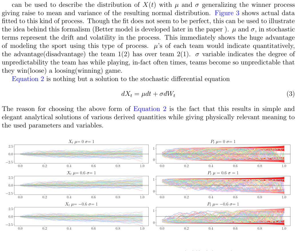
Summary. The manuscript introduces three stochastic differential equation (SDE) models for cricket, using the variable X(t) defined as the difference between net run rate and required run rate, and derives expressions for the win probability P(X(1)>0 | X(t)=alpha). Model 1 is Brownian motion with drift; Model 2 adds a wicket-dependent drift via a Poisson survival function; Model 3 is an Ornstein-Uhlenbeck process with parameters (x0, x1, sigma) intended to summarize team quality. The paper illustrates the models on a historic India-Sri Lanka ODI and proposes the parameter triplet as a quantitative team descriptor.

Significance. The conceptual idea of modelling cricket's score differential by an SDE is reasonable and could lead to a compact, interpretable team descriptor and a ball-by-ball win-probability update. The manuscript provides explicit formulas and a clear framework, which is a useful starting point. However, the central probability formulas contain algebraic errors (Eqs. 4, 6, and 15), the variance expression in Eq. 7 is not derived and appears malformed, the reported fit includes a negative volatility, and the illustrative match is inside the fitting period, so the quantitative claims are not supported as written.

major comments (5)

[2.1, Eqs. (4) and (6)] For X(1) ~ N(mu, sigma^2), the correct win probability is P(X(1)>0) = 1/2[1 + erf(mu/(sigma sqrt(2)))]. Equation (4) instead has (1 - mu) in the numerator, which is dimensionally wrong and numerically incorrect (e.g., at mu=0 it gives a value depending on 1/sigma rather than 1/2). Similarly, Eq. (6), the conditional probability given X(t1)=alpha, should be 1/2[1 + erf((alpha + mu(1-t1))/(sigma sqrt(2(1-t1))))], but the printed formula contains '1 - mu(1-t1) - alpha', which has the wrong sign structure and is not monotone increasing in alpha as it should be. These errors invalidate the Model 1 probability curves shown in Figures 2 and 5.
[2.1, Eq. (7)] The claimed 'closed form solution for the variance of the above probability' is introduced with 'After few steps of calculations' and is not derived. The expression mixes a probability-like term with Owen's T function without defining the random variable over which the variance is taken, and it states independence of alpha even though the probability in Eq. (6) depends on alpha. As written, Eq. (7) cannot be checked, reproduced, or used; it should either be derived rigorously with all assumptions stated, or removed.
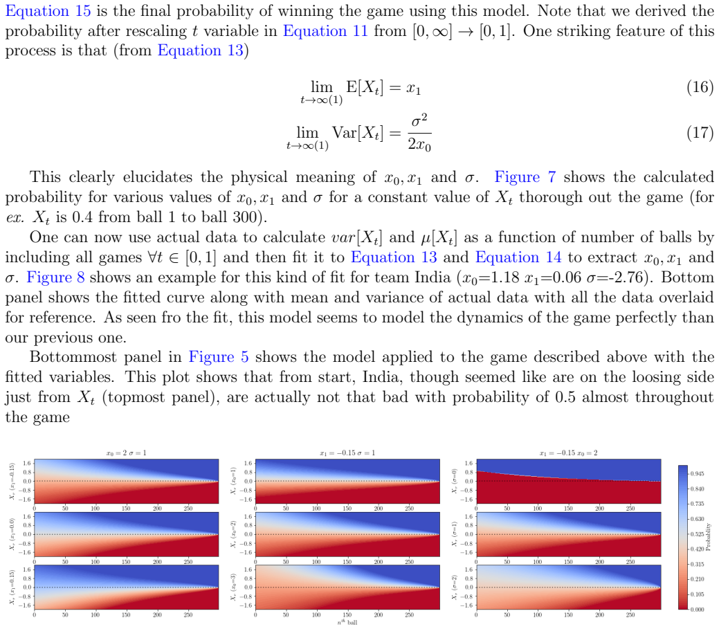
[2.3, Eq. (15)] Equation (15) is the central formula of the paper, giving P(X(1)>0 | X(t)=alpha) for the Ornstein-Uhlenbeck process dX_t = x0(x1-X_t)dt + sigma dW_t. For this process, the conditional distribution is normal with mean m = alpha e^{-x0(1-t)} + x1(1-e^{-x0(1-t)}) and variance v = sigma^2/(2x0)(1-e^{-2x0(1-t)}), so the correct probability is 1/2[1 + erf(m/sqrt(2v))]. The printed Eq. (15) has an extra factor sqrt(2), places x1 inside an exponential multiplying alpha, and omits the x1(1-e^{-x0(1-t)}) term; it does not reduce to the correct expression even in the case x1=0. For example, with x0=1, x1=0, sigma=1, alpha=1, and t=0, the correct OU value is about 0.71, while Eq. (15) interpreted literally gives about 0.80. Because this formula underlies the win-probability panels in Figures 5, 7, and 9, the central quantitative claim is unsupported by the manuscript as written.
[2.3, Fig. 8] The reported fit for team India gives sigma = -2.76. Since Eq. (14) depends on sigma^2 and Eq. (15) uses sigma in the denominator of an erf argument, a negative value is not a harmless sign convention: it would flip the sign of the probability correction and contradicts the stated interpretation of sigma as a volatility. The paper must report a nonnegative sigma (or explicitly define a signed convention and justify it), and should provide parameter uncertainties; without this, the fitted triplet (x0, x1, sigma) is not physically meaningful.
[2.3, Figs. 5 and 8] The illustrative India-Sri Lanka match (April 2, 2011) lies inside the 2005-2017 period used to fit x0, x1, and sigma for India (Fig. 8). Therefore the win-probability curves in Figures 5, 7, and 9 are in-sample evaluations, not predictions. The abstract claims a method to calculate winning probability as a progression of balls, but no out-of-sample test is provided; a demonstration such as fitting on pre-2011 data and evaluating on later matches is needed to support the predictive claim.

minor comments (5)

[Section 1, Eq. (1) and Conclusion] The definition of X(t) is inconsistent: Eq. (1) defines X(t) = NR(t) - RR(t), while the Conclusion states 'Xt := RR - NR'; this sign discrepancy must be resolved throughout the paper.
[Abstract and throughout] There are numerous typographical errors, including 'statical cumulants' (Abstract), 'winner process' (Section 2.1, should be 'Wiener process'), and repeated 'loosing' for 'losing'. These should be corrected in a thorough revision.
[2.1, Eq. (2)] The notation is inconsistent: Eq. (2) writes N(mu t, sigma^2 t), using sigma^2 as a variance, while later the text and Eq. (4) write N(mu, sigma), with sigma as a standard deviation. Standardize the notation to avoid confusion.
[2.3, Eq. (11)] Equation (11) is missing parentheses: it should read dX_t = x0(x1 - X_t)dt + sigma dW_t. As printed, 'dXt = x0x1 - x0Xtdt + sigma dWt' is ambiguous.
[2.3, Eqs. (12) and (13)] Equations (12) and (13) use X_{t-1} as the initial value, but the solution of the OU process from time 0 should involve X_0; the notation should be corrected and the time indices made consistent.

Circularity Check

0 steps flagged · score 0.0 of 10

No significant circularity: the OU model and conditional win probability are derived from a stated stochastic ansatz, not from a self-citation or a fitted outcome variable.

full rationale

The derivation chain is self-contained. Model 3 posits dX_t = x0(x1-X_t)dt + sigma dW_t as an ansatz (Eq. 11), solves it (Eq. 12), and computes conditional mean and variance (Eqs. 13-14) by standard OU calculus. Eq. 15 is then presented as the resulting conditional win probability; whether it is algebraically correct is a separate question from circularity. The parameters x0, x1, sigma are fitted to historical mean and variance curves of X_t (Figure 8), and the win probability is a deterministic transformation of those fitted parameters, not a parameter fitted directly to win/loss outcomes. The illustrative India-Sri Lanka match is inside the fitting period, so the displayed probability curves are in-sample backcasts rather than out-of-sample predictions; this is a validation weakness, not a circular reduction. There are no self-citations, no uniqueness theorems imported from the authors, and no claim whose load-bearing premise is justified only by the authors' prior work. The paper's core steps do not reduce to their inputs by construction.

Assumptions & free parameters 7 free parameters · 5 assumptions · 1 invented entities

The model's output depends on seven fitted or estimated numbers (mu, sigma, mu_bar, w_bar, x0, x1, sigma) and several strong domain assumptions about game dynamics, wicket arrivals, and the transfer of historical parameters to new matches. No external validation, error bars, or out-of-sample tests are provided.

free parameters (7)

mu (Model 1 drift) = England: -0.2; England vs Pakistan: 0.17
Fitted to the distribution of final X_1 for England ODI games 2005-2017; no error bars or fitting procedure are reported.
sigma (Model 1 volatility) = England: 1.12
Fitted alongside mu to the normal curve in Figure 3.
mu_bar (Model 2 disadvantage factor) = not specified
Called a universal constant for the game in Eq. 10, but never estimated or given a value.
w_bar (average wickets lost) = India: 7.4
Empirical average wickets lost per game used in Model 2's Poisson survival function.
x0 (Model 3 reversion rate) = India: 1.18
Fitted from historical mean and variance curves for India 2005-2017 (Figure 8).
x1 (Model 3 long-run mean) = India: 0.06
Fitted along with x0 from the mean curve.
sigma (Model 3 volatility) = India: -2.76
Reported as a fitted volatility; a negative value is invalid for a diffusion coefficient and signals a fitting or reporting error.

assumptions (5)

domain assumption The game outcome is equivalent to X(1)>0, i.e., the chasing team wins exactly when the final net run rate exceeds the required run rate.
This ignores early termination, ties, super overs, and DLS adjustments; stated in section 2.1 around Eq. 4.
domain assumption X_t follows a Brownian motion with drift in Model 1 and an Ornstein-Uhlenbeck process in Model 3 with constant parameters.
The central modeling assumption in Eqs. 2, 3, and 11.
domain assumption Wicket arrivals follow a Poisson process with mean w_bar.
Stated explicitly in section 2.2: 'The assumption we have made here is that the fall of wickets follows a Poisson distribution.'
domain assumption Team-specific fitted parameters remain valid for a particular match and opponent.
Used when applying India-fitted x0, x1, sigma to the India-Sri Lanka match in Figure 5.
standard math Standard Brownian motion properties: W0=0, continuous paths, independent stationary increments.
Listed in section 2.1 to define W_t.

invented entities (1)

Disadvantage factor mu_bar
purpose: A universal constant modulating the drift reduction when wickets are lost (Eq. 10).
Postulated as a universal constant for cricket, but no value, estimation procedure, or external validation is given.

how reviews work

0 comments

Cite this review

Pith. "Pith review of Stochastic differential theory of cricket." pith.science (2026). https://pith.science/paper/7ZKGMX66

@misc{pith2026190807372,
  author       = {Pith},
  title        = {Pith review of: Stochastic differential theory of cricket},
  year         = {2026},
  howpublished = {\url{https://pith.science/paper/7ZKGMX66}},
  note         = {Machine review of arXiv:1908.07372}
}

read the original abstract

A new formalism for analyzing the progression of cricket game using Stochastic differential equation (SDE) is introduced. This theory enables a quantitative way of representing every team using three key variables which have physical meaning associated with them. This is in contrast with the traditional system of rating/ranking teams based on combination of different statical cumulants. Further more, using this formalism, a new method to calculate the winning probability as a progression of number of balls is given.

Figures

Figures reproduced from arXiv: 1908.07372 by the authors.

**Figure 1.** typical X(t) from a cricket match. Here it is shown for an ODI game and hence T = 300. Blue points represent every 4th ball and red line, the entire game. One can write the distribution of the lead of one team over an other team (X(t)) at any point in the game as a weinner process. Let (Wt)t≥0+ denotes a standard Brownian motion satisfying • W0 = 0 • With probability 1, the function t → Wt is continuous in t • The p… view at source ↗

**Figure 2.** Simulated trajectories of Equation 3 and their corresponding P(X(1)|X(t1) = Xt1 ) > 0 for various values of µ. Red shaded region shows the variance of each individual trajectories overlaid on each other. One of the important quantity we are interested in is PT := P(X(T) > 0). PT is the probability of the given path to reach a point above 0. This would mean that the NR is greater than RR at the end of the game, thus … view at source ↗

**Figure 3.** Actual distribution of team England of their last ball [PITH_FULL_IMAGE:figures/full_fig_p004_3.png] view at source ↗

Figures from the paper (6 more)

**Figure 4.** Figure 4: f( ¯w, wt) from Equation 10 for various mean wickets lost in a game [PITH_FULL_IMAGE:figures/full_fig_p006_4.png]

**Figure 6.** Figure 6: Distribution of actual wickets lost by team India from the period 2005 [PITH_FULL_IMAGE:figures/full_fig_p006_6.png]

**Figure 5.** Figure 5: Xt and Pt calculated using the models shown in the paper for a real game of India against Sri lanka (ICC Cricket World Cup at Mumbai, Apr 2 2011 ). Each vertical red line indicate the player getting out. Dotted area shows the variance and the confidence level of the ca…

**Figure 7.** Figure 7: Color map of Pt calculated for various values of x0, x1, σ for Equation 11 with Xt being constant across all balls. Dotted lines indicate Pt when Xt = 0 for all t. As mentioned earlier, this paper boils down to mapping Xt :→ Pt . Model 3 developed in subsection 2.3 ca…

**Figure 8.** Figure 8: Fit for mean and variance for team India using [PITH_FULL_IMAGE:figures/full_fig_p009_8.png]

**Figure 9.** Figure 9: Thick black and red curves shows the actual [PITH_FULL_IMAGE:figures/full_fig_p009_9.png]

Discussion (0). Continue with ORCID to comment.

Reference graph

Works this paper leans on

17 extracted references · 17 canonical work pages

[1]

Exploring limits to prediction in complex social systems

Martin, Travis, et al. “Exploring limits to prediction in complex social systems.” Proceedings of the 25th International Conference on World Wide Web. International World Wide Web Conferences Steering Committee, 2016

work page 2016
[2]

The implied volatility of a sports game

Polson, Nicholas G., and Hal S. Stern. “The implied volatility of a sports game.” Journal of Quantitative Analysis in Sports 11.3 (2015): 145-153

work page 2015
[3]

A Brownian motion model for the progress of sports scores

Stern, Hal S. “A Brownian motion model for the progress of sports scores.” Journal of the American Statistical Association 89.427 (1994): 1128-1134

work page 1994
[4]

Wei-Sen Chen and Yin-Kuan Du. 2009. Using neural networks and data mining techniques for the ﬁnancial distress prediction model. Expert Systems with Applications 36, 2 (2009), 40754086

work page 2009
[5]

Shuo Chen and Thorsten Joachims. 2016. Predicting matchups and preferences in context. In Proceedings of the 22nd ACM SIGKDD International Conference on Knowledge Discovery and Data Mining. ACM, ACM, USA, 775784

work page 2016
[6]

Dominique Haughton, Mark-David McLaughlin, Kevin Mentzer, and Changan Zhang. 2015. Oscar Prediction and Prediction Markets. In Movie Analytics. Springer, -, 3739

work page 2015
[7]

Andranik Tumasjan, Timm Oliver Sprenger, Philipp G Sandner, and Isabell M Welpe. 2010. Predicting elections with twitter: What 140 characters reveal about political sentiment. ICWSM 10, 1 (2010), 178185

work page 2010
[8]

Park, J. and M. E. J. Newman Journal of Statistical Mechanics : Theory and Exper- iment,

work page

Show all 17 references

[9]

Mukherjee, Physica A 391, 6066 (2012)

S. Mukherjee, Physica A 391, 6066 (2012)

2012
[10]

Increased Prediction Accuracy in the Game of Cricket using Machine Learning

Passi, Kalpdrum, and Niravkumar Pandey. “Increased Prediction Accuracy in the Game of Cricket using Machine Learning.” arXiv preprint arXiv:1804.04226 (2018)

2018 arXiv
[11]

Stochastic volatility with an OrnsteinUhlenbeck process: an extension

Schobel, Rainer, and Jianwei Zhu. “Stochastic volatility with an OrnsteinUhlenbeck process: an extension.” Review of Finance 3.1 (1999): 23-46

1999
[12]

Quantifying individual performance in Cricket - A network analysis of batsmen and bowlers,

S. Mukherjee, “Quantifying individual performance in Cricket - A network analysis of batsmen and bowlers,” Physica A: Statistical Mechanics and its Applications, vol. 393, pp. 624-637, 2014. 10

2014
[13]

Analysis of Performance of Bowlers using Combined Bowling Rate,

D. Bhattacharjee and D. G. Pahinkar, “Analysis of Performance of Bowlers using Combined Bowling Rate,” International Journal of Sports Science and Engineering, vol. 6, no. 3, pp. 1750-9823, 2012

2012
[14]

Quantifying individual performance in Cricket - A network analysis of batsmen and bowlers,

S. Mukherjee, “Quantifying individual performance in Cricket - A network analysis of batsmen and bowlers,” Physica A: Statistical Mechanics and its Applications, vol. 393, pp. 624-637, 2014

2014
[15]

New performance measure in Cricket,

P. Shah, “New performance measure in Cricket,” ISOR Journal of Sports and Physical Educa- tion, vol. 4, no. 3, pp. 28-30, 2017

2017
[16]

Player valuations in the Indian Premier League,

D. Parker, P. Burns and H. Natarajan, “Player valuations in the Indian Premier League,” Frontier Economics, vol. 116, October 2008

2008
[17]

A Mathematical Modelling Approach to One-Day Cricket Batting Orders,

M. Ovens and B. Bukiet, “A Mathematical Modelling Approach to One-Day Cricket Batting Orders,” Journal of Sports Science and Medicine, vol. 5, pp. 495-502, 15 December 2006. 11

2006

Pith tools

Reviewed August 14, 2026 · model on record in the stance chip above.

[1] [1]

Exploring limits to prediction in complex social systems

Martin, Travis, et al. “Exploring limits to prediction in complex social systems.” Proceedings of the 25th International Conference on World Wide Web. International World Wide Web Conferences Steering Committee, 2016

work page 2016

[2] [2]

The implied volatility of a sports game

Polson, Nicholas G., and Hal S. Stern. “The implied volatility of a sports game.” Journal of Quantitative Analysis in Sports 11.3 (2015): 145-153

work page 2015

[3] [3]

A Brownian motion model for the progress of sports scores

Stern, Hal S. “A Brownian motion model for the progress of sports scores.” Journal of the American Statistical Association 89.427 (1994): 1128-1134

work page 1994

[4] [4]

Wei-Sen Chen and Yin-Kuan Du. 2009. Using neural networks and data mining techniques for the ﬁnancial distress prediction model. Expert Systems with Applications 36, 2 (2009), 40754086

work page 2009

[5] [5]

Shuo Chen and Thorsten Joachims. 2016. Predicting matchups and preferences in context. In Proceedings of the 22nd ACM SIGKDD International Conference on Knowledge Discovery and Data Mining. ACM, ACM, USA, 775784

work page 2016

[6] [6]

Dominique Haughton, Mark-David McLaughlin, Kevin Mentzer, and Changan Zhang. 2015. Oscar Prediction and Prediction Markets. In Movie Analytics. Springer, -, 3739

work page 2015

[7] [7]

Andranik Tumasjan, Timm Oliver Sprenger, Philipp G Sandner, and Isabell M Welpe. 2010. Predicting elections with twitter: What 140 characters reveal about political sentiment. ICWSM 10, 1 (2010), 178185

work page 2010

[8] [8]

Park, J. and M. E. J. Newman Journal of Statistical Mechanics : Theory and Exper- iment,

work page