A lognormal type stochastic volatility model with quadratic drift

Peter Carr; Sander Willems

REVIEW 3 major objections 5 minor 41 references

A lognormal type stochastic volatility model with quadratic drift

T0 review · 3 major / 5 minor · reviewed 2026-08-14 · deepseek-v4-flash

Challenge this review Re-run · record.json Download PDF Read on arXiv ↗ Review JSON

Pith's one-line read A quadratic drift term in the volatility process is what keeps the stock price a martingale and higher moments finite, the paper argues, while a change of measure makes option pricing fast.

desk verdict A genuinely new quadratic-drift stochastic volatility model with clean martingale/moment results and a useful measure-change trick; the pricing approximation is promising but the 'highly accurate' claim outruns the numerical evidence. read the letter →

arxiv 1908.07417 v1 pith:4UYQA2JU submitted 2019-08-20 q-fin.MF q-fin.CPq-fin.PRq-fin.RM

Peter Carr , Sander Willems This is my paper · ORCID

classification q-fin.MFq-fin.CPq-fin.PRq-fin.RM MSC 91G2060H1060J60

keywords stochasticvolatilityquadraticdriftmomentexplosionmartingalepropertypolynomialdiffusionGeneralizedInverseGaussiandistributionorthogonalexpansionoptionpricing

verification ladder T0 review T1 audit T2 compute T3 formal

The pith

A machine-rendered reading of the paper's core claim, the machinery that carries it, and where it could break.

The reading

This paper proposes a one-factor stochastic volatility model in which volatility follows a diffusion with a quadratic drift and a linear dispersion function. The authors argue that the quadratic term, controlled by the parameter $R_1$, is what prevents the moment explosions and loss of martingality that typically plague lognormal-type volatility models. A carefully chosen change of measure then turns the volatility process into a polynomial diffusion, so all conditional moments become available in closed form. The payoff is a non-affine model with an empirically supported stationary GIG distribution that still supports fast, deterministic option pricing.

What carries the argument

The engine is the change of measure (7), where $y_t$ is defined by $dy_t = -\frac12 z^2 \sigma_t^2 dt + z\sigma_t dW_t$ with $z = R_1/\nu$. Under $\mathbb{Q}^z$, the volatility process has affine drift and linear dispersion, so it is a polynomial diffusion, and the augmented state $(x_t, y_t, \sigma_t, \sigma_t^2)$ is jointly polynomial. The generator matrices $G_m$ are built by collecting monomial terms, giving the moment formula $\mathbb{E}_t^z[H_m(x_T,y_T,\sigma_T)] = e^{G_m(T-t)}H_m(x_t,y_t,\sigma_t)$. Pricing then projects the discounted payoff onto orthogonal polynomials using a Gaussian-mixture auxiliary density $w$ obtained from the IJK discretization scheme and Gauss-Hermite quadrature, with a recursive formula for call-option integrals.

What would settle it

Take a maturity well beyond the two months tested, for example $T = 1$ year, with a positive correlation $\rho$ and $R_1$ only slightly above $\rho\nu$; compute $\pi_n$ for $n$ up to 15 and compare against a high-precision Monte Carlo estimate with $10^7$ paths and a control variate. If the polynomial prices leave the Monte Carlo confidence band or fail to settle as $n$ grows, the auxiliary-density proxy is not adequate for that regime. Alternatively, simulate (1)-(2) with $R_1 < \rho\nu$ and check whether sample moments $\mathbb{E}[S_T^m]$ diverge as predicted, which would confirm the threshold condition.

Watch

Extended reading notes

Core claim

The central claim is that, for the dynamics (1)-(2), the condition $R_1 \geq \rho\nu$ is necessary and sufficient for the discounted stock price $S_t$ to be a martingale, and that for each moment order $m$, $R_1 > \nu(\rho m + \sqrt{m^2 - m})$ guarantees $\mathbb{E}_t[S_T^m] < \infty$ for all $T$. The quadratic drift thus takes over the stabilizing role that strong negative correlation plays in affine models, leaving $\rho$ as a free parameter. Under the measure change $d\mathbb{Q}^z/d\mathbb{Q} = e^{y_T}$ with $z = R_1/\nu$, the volatility drift becomes affine and the augmented process $(x_t, y_t, \sigma_t, \sigma_t^2)$ becomes a polynomial diffusion under $\mathbb{Q}^z$. Consequently, all conditional moments are given by matrix exponentials, and European option prices are approximated by projecting the discounted payoff $e^{-y}F(e^x)$ onto bivariate polynomials, yielding $\pi_n = \vec{p}_n^\top e^{G_n T} H_n(x_0, y_0, \sigma_0)$.

Load-bearing premise

The pricing approximation is accurate only if the Gaussian-mixture auxiliary density $w$ built from the discretized IJK scheme faithfully proxies the true $\mathbb{Q}^z$-distribution of $(x_T, y_T)$; the authors provide numerical evidence but no error bound, and they note that too few quadrature points ($K=3$) makes the approximation blow up.

Editorial extensions

If this is right

If $R_1 \geq \rho\nu$, the model supports positive correlation between returns and volatility while preserving the martingale property, widening the usable parameter space beyond the negative-correlation requirement of affine models.
The closed-form critical moments $m_\pm$ in Corollary 4.3, combined with Lee's moment formula, give explicit control over both small- and large-strike implied volatility slopes, which can be used for calibration.
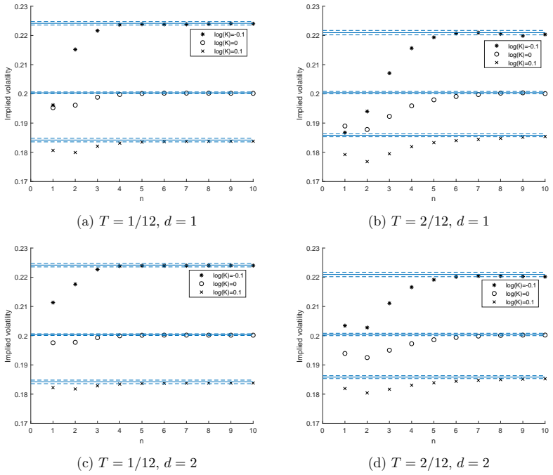
European option prices can be computed deterministically via the polynomial expansion; in the tested one- and two-month maturities, $\pi_n$ converges to within Monte Carlo confidence bands with $n \leq 10$.
The stationary distribution is a Generalized Inverse Gaussian, which nests gamma and inverse-gamma cases and matches empirical evidence on volatility dynamics.

Reading between the lines

Editorial extensions of the paper, not claims the author makes directly.

Beyond the paper's numerical tests, the same measure-change construction might apply to other non-polynomial diffusions with a quadratic drift, suggesting a general recipe for embedding such models into the polynomial class.
The reported blow-up for $K=3$ indicates that the pricing method's reliability depends on the auxiliary density having sufficiently heavy tails; adaptive or quantile-based quadrature rules could extend accuracy to parameter regimes where the Gaussian-mixture proxy is thin-tailed.
If the time-horizon independence of the critical moments holds beyond the presented proofs, the model predicts implied-volatility smile asymptotics that are stationary across maturities, a directly testable empirical signature.
The boundedness results for $\rho = \pm 1$ in Proposition 4.5 could be exploited to generate hard no-arbitrage bounds on derivative prices, useful as control variates in Monte Carlo.

Share X Bluesky LinkedIn Reddit HN

Signed reviews

No signed human review yet.

Editorial analysis

A structured set of objections, weighed in public.

Desk editor's note, referee report, and a circularity audit.

Desk Editor's Note

read the letter

Dear colleague,

Short version: this is a real contribution to the stochastic volatility toolbox, and the core math holds up. The paper writes down the one-factor model dxt = -1/2 sigma^2 dt + sigma(rho dW + sqrt(1-rho^2) dB), dsigma = (R0+R1 sigma)(R2-sigma) dt + nu sigma dW, with R0,R1 >= 0. The fully general quadratic drift case appears to be new; the nesting table in Section 2 is useful. The important results are Propositions 4.1 and 4.2: the stock is a true martingale if and only if R1 >= rho nu, and finite m-th moments hold under an explicit lower bound on R1. Those criteria are clean, and the proofs in the appendix are standard and sound. The GIG steady-state derivation (Prop 3.1) is also correct and nicely ties together the inverse gamma and gamma special cases. The measure change in Section 5 is the elegant centerpiece: with z = R1/nu, under Q^z the volatility drift becomes affine, and the generator of (x,y,sigma,sigma^2) becomes polynomial. That is a neat trick that lets the authors compute joint Q^z moments in closed form.

The pricing method that follows — orthogonal projection of e^{-y}F(e^x) onto bivariate polynomials weighted by a Gaussian-mixture auxiliary density, then applying the generator matrix exponential — is a sensible extension of Ackerer–Filipovic. But this is where the paper gets soft. The auxiliary density w in Eq. (13) is a heuristic discretization of the unknown Q^z density: K samples from the IJK path discretization and Gauss-Hermite quadrature. The authors themselves report that K=3 blows up for larger n, and they give no error bound or convergence statement as n, K, and the number of time steps d vary. The numerical section covers one parameter set, two maturities (up to 2 months), and three strikes within +/-10%. That is not enough to support the abstract's 'highly accurate' claim. It is probably accurate for the tested cases, but the method might degrade for longer maturities or different parameters, especially with the single time-step variant.

Everything else looks solid to me. The citation pattern is appropriate; Lions–Musiela, Andersen–Piterbarg, Lee, and Filipovic–Larsson are all cited where the arguments need them. The empirical Figure 1 is illustrative rather than evidence, but it is not load-bearing. The paper is honestly written: it flags the K=3 problem itself and notes the Lions–Musiela typos in the appendix.

Who is this for? Anyone working on tractable non-affine stochastic volatility models. It gives a new model with explicit martingale/moment conditions and a fast pricing route. It deserves a serious referee. My recommendation: send it out, but ask for either an error analysis or a broader numerical study before the 'highly accurate' claim stands. As is, I would cite it for the model and the moment bounds, with a caveat on the pricing numerics.

Best, [You]

Referee Report

3 major / 5 minor

Summary. The paper introduces a one-factor stochastic volatility model in which the log-price x_t follows (1) and the volatility σ_t follows (2) with quadratic drift (R0 + R1σ)(R2 − σ) and linear dispersion νσ. It proves existence, uniqueness, and zero-unattainability of the solution (Proposition 2.1), derives the GIG steady-state density (Proposition 3.1), gives necessary and sufficient martingale and moment-explosion conditions (Propositions 4.1 and 4.2), computes the Lee critical moments (Corollary 4.3), and introduces a change of measure dQ^z/dQ = e^{y_T} under which the joint process (x_t, y_t, σ_t) becomes polynomial-like (Proposition 5.3). It then proposes an option pricing method that replaces the unknown Q^z density of (x_T, y_T) by an auxiliary Gaussian-mixture/delta density w, projects the discounted payoff onto bivariate polynomials, and tests the approximation numerically in Section 7.

Significance. If the model-level results hold, this is a useful contribution: it gives a non-affine one-factor stochastic volatility model with a stationary GIG distribution, explicit control of moment explosions via the quadratic drift, closed-form conditional moments under a measure change, and a concrete mapping from model parameters to implied-volatility tail slopes via the Lee formula. The martingale, moment, and steady-state derivations are carefully argued and appear correct, and Proposition 5.3 is a clean result. The pricing approximation is the main uncertainty: it is heuristic, relies on an auxiliary density with finite support, and is validated only on a single parameter set. With additional numerical validation or an error bound, the pricing contribution could be made solid; as it stands, the 'highly accurate' claim is not yet supported.

major comments (3)

[Section 7] The numerical study uses exactly one parameter set (R0 = R1 = 5, ν = 1, R2 = σ0 = 0.20, ρ = -0.5), maturities T ∈ {1/12, 2/12}, and strikes log K ∈ {-0.1, 0, 0.1}. This is too narrow to support the abstract's 'highly accurate option price approximation technique' claim. The error mechanism depends on how well the auxiliary density w in Eq. (13) reproduces the true Q^z distribution of (x_T, y_T), and that distribution depends strongly on the parameters and on T; in particular, regimes near the martingale boundary R1 = ρν and large |ρ| are untested. I ask for either an error bound or a systematic numerical study across maturities, strikes, and parameter regions, with reported absolute price errors.
[Section 6.2, Eq. (13)] The auxiliary density w has Dirac components in y, so the least-squares projection (11) only controls the polynomial p_n at the K quadrature values y^(k). There is no control of the error in E^{Q^z}[p_n(X_T, Y_T)] under the true continuous distribution of Y_T, and no convergence statement is given as K, d, and n vary. The paper's own report that K = 3 makes the approximation blow up (Section 7) shows that this failure mode is real. Since the price π_n in Eq. (12) combines coefficients computed from w with moments computed under Q^z, this gap is load-bearing for the pricing claim.
[Section 7, d = 1 vs d = 2] The comparison between d = 1 and d = 2 is not controlled: the former uses K = 15 quadrature points, while the latter uses K = 225 (or 185 after pruning), so the faster convergence displayed in Figures 3c and 3d could be due to the larger K rather than to the finer time discretization. The paper should separate the effects of K and d in order to support the statement that increasing d improves the approximation.

minor comments (5)

[Title page and Section 3] The title page and abstract contain the typo 'quadrati c drift', and Section 3 contains 'exponential decay of of the left tail'.
[Section 5 and Proposition 5.3] The symbol z is used both for the constant R1/ν (Eqs. 6-7) and as the third state variable in the polynomial space P_m (e.g., Eq. 22). This makes the generator formula harder to read; please rename one of the two uses.
[Appendix A.2] In the proof of Proposition 3.1, the sentence 'If 2R1R2 ≥ ν^2, then e^{(R1R2 - 1/2 ν^2)t + νW_t} → 0' has the inequality direction reversed; the convergence to zero occurs when 2R1R2 ≤ ν^2, consistent with Proposition 3.1.
[Eq. (22)] Equation (22) formally contains monomials with negative powers when any of α, β, or γ is zero; please state the convention that terms with negative exponents are omitted or otherwise clarify the formula's domain.
[Appendix B.1] The line 'β − −2R1/ν^2' contains a double minus sign; this appears to be a typo for β = -2R1/ν^2.

Circularity Check

0 steps flagged · score 0.0 of 10

No significant circularity: the model-level results are derived from external theorems and the pricing approximation is checked against independent Monte Carlo, not against fitted inputs.

full rationale

The paper's derivation chain is self-contained and non-circular. The martingale and moment criteria in Propositions 4.1 and 4.2 are obtained by applying the externally stated Lions and Musiela (2007) theorems, with the required limit calculations carried out in the appendix; Proposition 4.2 is then used to derive the critical moments in Corollary 4.3. The GIG steady-state distribution in Proposition 3.1 comes from solving the Fokker-Planck equation with an explicit ansatz, not from imposing the target distribution. The change of measure in Section 5 is justified by a martingale proof using the same external criterion, and the polynomial-moment formula in Proposition 5.3 is proved directly from the generator action on monomials. The pricing method in Section 6 is an approximation: the auxiliary density w in Eq. (13) is a quadrature-based proxy, and the polynomial projection in Eq. (11) is evaluated against a Monte Carlo benchmark in Section 7, so the numerical prices are not fitted to reproduce the benchmark. The only self-citations (Willems 2019; Filipovic and Willems 2017) appear as background references in the introduction and are not load-bearing for any result. The acknowledged K=3 blow-up and the absence of error bounds are numerical limitations, not circularity, because the approximation is not asserted to be an identity obtained from its own inputs.

Assumptions & free parameters 0 free parameters · 5 assumptions · 0 invented entities

The model parameters R0, R1, R2, ν, ρ, σ0 are inputs rather than fitted values, so no data-fitted free parameters appear. The paper relies on standard stochastic calculus results and on an unproven adequacy of the auxiliary density for the pricing approximation.

assumptions (5)

domain assumption R0 >= 0 and R1 >= 0 are assumed; R1 < 0 leads to finite-time blow-up.
The model specification (Section 2) constrains R0 and R1 to be nonnegative. Remark A.1 shows this is necessary for a global solution, so it is a load-bearing modeling choice, not an empirical finding.
standard math Lions and Musiela (2007) Theorems 2.4-2.6 provide the martingale and moment criteria used in Propositions 4.1, 4.2, and 5.1.
These external results are applied without proof. The paper even notes typos in the source, so the acceptance of these criteria is taken on faith in the prior theorem. If the criteria were incorrect, the moment explosion results would fail.
standard math The Fokker-Planck equation gives the steady-state density of σ_t; normalization uses known GIG density constants (Jorgensen 1982).
Standard PDE approach; the Ansatz in A.2 relies on known gamma and inverse-gamma special cases to fix the form.
standard math Girsanov's theorem applies under Qz because e^{y_T} is a true Q-martingale (Proposition 5.1).
The change of measure is valid only if the Radon-Nikodym derivative is a martingale, which the paper proves by invoking Lions-Musiela. This is standard stochastic calculus.
ad hoc to paper The auxiliary density w in Eq. (13) is a valid probability density and the weighted L2 projection (11) has a unique solution.
The paper assumes the Gaussian-mixture weight makes the projection well-defined and accurate; no approximation guarantee is proven. Section 6.2 says the weight proxies the unknown Qz density, and the numerical study shows sensitivity to K.

how reviews work

0 comments

Cite this review

Pith. "Pith review of A lognormal type stochastic volatility model with quadratic drift." pith.science (2026). https://pith.science/paper/4UYQA2JU

@misc{pith2026190807417,
  author       = {Pith},
  title        = {Pith review of: A lognormal type stochastic volatility model with quadratic drift},
  year         = {2026},
  howpublished = {\url{https://pith.science/paper/4UYQA2JU}},
  note         = {Machine review of arXiv:1908.07417}
}

read the original abstract

This paper presents a novel one-factor stochastic volatility model where the instantaneous volatility of the asset log-return is a diffusion with a quadratic drift and a linear dispersion function. The instantaneous volatility mean reverts around a constant level, with a speed of mean reversion that is affine in the instantaneous volatility level. The steady-state distribution of the instantaneous volatility belongs to the class of Generalized Inverse Gaussian distributions. We show that the quadratic term in the drift is crucial to avoid moment explosions and to preserve the martingale property of the stock price process. Using a conveniently chosen change of measure, we relate the model to the class of polynomial diffusions. This remarkable relation allows us to develop a highly accurate option price approximation technique based on orthogonal polynomial expansions.

Figures

Figures reproduced from arXiv: 1908.07417 by the authors.

**Figure 2.** Simulated trajectory for σt with parameters R0 = R1 = 5, R2 = σ0 = 0.20, ν = 1. skewed (ρ < 0). Therefore, approximations which do not take into account at least third order moments will be far off for low strike options. The results are robust to changes in the number of discretization points K, as long as it is not too small. If K is chosen very small (say, K = 3), then the approximation blows up for larger n. Int… view at source ↗

**Figure 3.** Black-Scholes implied volatilities of approxima [PITH_FULL_IMAGE:figures/full_fig_p014_3.png] view at source ↗

Discussion (0). Continue with ORCID to comment.

Reference graph

Works this paper leans on

41 extracted references · 40 canonical work pages

[1]

Ackerer, D. and D. Filipovi \'c (2016). Linear credit risk models. arXiv preprint arXiv:1605.07419\/

arXiv 2016
[2]

Ackerer, D. and D. Filipovi \'c (2019). Option pricing with orthogonal polynomial expansions. Mathematical Finance\/ , Forthcoming

work page 2019
[3]

Filipovi \'c , and S

Ackerer, D., D. Filipovi \'c , and S. Pulido (2018). The J acobi stochastic volatility model. Finance and Stochastics\/ 22\/ (3), 667--700

work page 2018
[4]

Andersen, L. B. and V. V. Piterbarg (2007). Moment explosions in stochastic volatility models. Finance and Stochastics\/ 11\/ (1), 29--50

work page 2007
[5]

Andersen, T. G., T. Bollerslev, F. X. Diebold, and H. Ebens (2001). The distribution of realized stock return volatility. Journal of Financial Economics\/ 61\/ (1), 43--76

work page 2001
[6]

Andersen, T. G., T. Bollerslev, F. X. Diebold, and P. Labys (2001). The distribution of realized exchange rate volatility. Journal of the American Statistical Association\/ 96\/ (453), 42--55

work page 2001
[7]

Ju, and H

Bakshi, G., N. Ju, and H. Ou-Yang (2006). Estimation of continuous-time models with an application to equity volatility dynamics. Journal of Financial Economics\/ 82\/ (1), 227--249

work page 2006
[8]

Barndorff-Nielsen, O. E. (1997). Normal inverse G aussian distributions and stochastic volatility modelling. Scandinavian Journal of statistics\/ 24\/ (1), 1--13

work page 1997

Show all 41 references

[9]

Rasmussen, and C

Barone-Adesi, G., H. Rasmussen, and C. Ravanelli (2005). An option pricing formula for the GARCH diffusion model. Computational Statistics & Data Analysis\/ 49\/ (2), 287--310

2005
[10]

Jacobs, and K

Christoffersen, P., K. Jacobs, and K. Mimouni (2010). Volatility dynamics for the S&P500 : evidence from realized volatility, daily returns, and option prices. The Review of Financial Studies\/ 23\/ (8), 3141--3189

2010
[11]

Filipovi \'c , W

Duffie, D., D. Filipovi \'c , W. Schachermayer, et al. (2003). Affine processes and applications in finance. The Annals of Applied Probability\/ 13\/ (3), 984--1053

2003
[12]

Eberlein, E. (2001). Application of generalized hyperbolic L\'e vy motions to finance. In L\'e vy processes , pp.\ 319--336. Springer

2001
[13]

Eberlein, E. and K. Prause (2002). The generalized hyperbolic model: financial derivatives and risk measures. In Mathematical Finance - Bachelier Congress 2000 , pp.\ 245--267. Springer

2002
[14]

Ewald, C.-O. and Z. Yang (2007). Geometric mean reversion: formulas for the equilibrium density and analytic moment matching. Available at SSRN 999561\/

2007
[15]

Gourier, and L

Filipovi \'c , D., E. Gourier, and L. Mancini (2016). Quadratic variance swap models. Journal of Financial Economics\/ 119\/ (1), 44--68

2016
[16]

Filipovi \'c , D. and M. Larsson (2016). Polynomial diffusions and applications in finance. Finance and Stochastics\/ 20\/ (4), 931--972

2016
[17]

Filipovi \'c , D. and S. Willems (2017). A term structure model for dividends and interest rates. Working Paper\/

2017
[18]

Gander, M. P. and D. A. Stephens (2007). Stochastic volatility modelling in continuous time with general marginal distributions: Inference, prediction and model selection. Journal of Statistical Planning and Inference\/ 137\/ (10), 3068--3081

2007
[19]

Hagan, P. S., D. Kumar, A. S. Lesniewski, and D. E. Woodward (2002). Managing smile risk. The Best of Wilmott\/ 1 , 249--296

2002
[20]

Heston, S. L. (1993). A closed-form solution for options with stochastic volatility with applications to bond and currency options. The Review of Financial Studies\/ 6\/ (2), 327--343

1993
[21]

Hull, J. and A. White (1987). The pricing of options on assets with stochastic volatilities. The Journal of Finance\/ 42\/ (2), 281--300

1987
[22]

Ikeda, N. and S. Watanabe (1989). Stochastic Differential Equations and Diffusion Processes\/ (2nd ed.), Volume 24. Elsevier

1989
[23]

J \"a ckel, P. (2005). A note on multivariate gauss-hermite quadrature. Technical report\/

2005
[24]

Jorgensen, B. (1982). Statistical Properties of the Generalized Inverse Gaussian Distribution , Volume 9. Springer Science & Business Media

1982
[25]

Kahl, C. and P. J \"a ckel (2006). Fast strong approximation monte carlo schemes for stochastic volatility models. Quantitative Finance\/ 6\/ (6), 513--536

2006
[26]

Karasinski, P. and A. Sepp (2012). Beta stochastic volatility model. Risk\/ , 66--71

2012
[27]

Karatzas, I. and S. Shreve (1991). Brownian Motion and Stochastic Calculus\/ (2nd ed.). Springer-Verlag

1991
[28]

Keller-Ressel, M. (2011). Moment explosions and long-term behavior of affine stochastic volatility models. Mathematical Finance: An International Journal of Mathematics, Statistics and Financial Economics\/ 21\/ (1), 73--98

2011
[29]

Kloeden, P. E. and E. Platen (1995). Numerical Solution of Stochastic Differential Equations , Volume 23. Springer Science & Business Media

1995
[30]

Zhu, et al

Lee, G., Z. Zhu, et al. (2016). Switching to non-affine stochastic volatility: A closed-form expansion for the I nverse G amma model. Technical report

2016
[31]

Lee, R. W. (2004). The moment formula for implied volatility at extreme strikes. Mathematical Finance\/ 14\/ (3), 469--480

2004
[32]

Lewis, A. L. (2000). Option Valuation Under Stochastic Volatility: With Mathematica Code . Finance Press

2000
[33]

Lewis, A. L. (2019). Exact solutions for a GBM -type stochastic volatility model having a stationary distribution. arXiv preprint arXiv:1809.08635\/

2019 arXiv
[34]

Lions, P.-L. and M. Musiela (2007). Correlations and bounds for stochastic volatility models. In Annales de l'Institut Henri Poincare (C) Non Linear Analysis , Volume 24, pp.\ 1--16. Elsevier

2007
[35]

Merton, R. C. (1975). An asymptotic theory of growth under uncertainty. The Review of Economic Studies\/ 42\/ (3), 375--393

1975
[36]

Nelson, D. B. (1990). ARCH models as diffusion approximations. Journal of Econometrics\/ 45\/ (1-2), 7--38

1990
[37]

Pag \`e s, G. and J. Printems (2003). Optimal quadratic quantization for numerics: the G aussian case. Monte Carlo Methods and Applications\/ 9\/ (2), 135--165

2003
[38]

Sepp, A. (2014). Empirical calibration and minimum-variance delta under log-normal stochastic volatility dynamics. Available at SSRN 2387845\/

2014
[39]

Sepp, A. (2016). Log-normal stochastic volatility model: Affine decomposition of moment generating function and pricing of vanilla options

2016
[40]

Tuckwell, H. C. and J. A. Koziol (1987). Logistic population growth under random dispersal. Bulletin of Mathematical Biology\/ 49\/ (4), 495--506

1987
[41]

Willems, S. (2019). Asian option pricing with orthogonal polynomials. Quantitative Finance\/ 19\/ (4), 605--618

2019

Pith tools

Reviewed August 14, 2026 · model on record in the stance chip above.

[1] [1]

Ackerer, D. and D. Filipovi \'c (2016). Linear credit risk models. arXiv preprint arXiv:1605.07419\/

arXiv 2016

[2] [2]

Ackerer, D. and D. Filipovi \'c (2019). Option pricing with orthogonal polynomial expansions. Mathematical Finance\/ , Forthcoming

work page 2019

[3] [3]

Filipovi \'c , and S

Ackerer, D., D. Filipovi \'c , and S. Pulido (2018). The J acobi stochastic volatility model. Finance and Stochastics\/ 22\/ (3), 667--700

work page 2018

[4] [4]

Andersen, L. B. and V. V. Piterbarg (2007). Moment explosions in stochastic volatility models. Finance and Stochastics\/ 11\/ (1), 29--50

work page 2007

[5] [5]

Andersen, T. G., T. Bollerslev, F. X. Diebold, and H. Ebens (2001). The distribution of realized stock return volatility. Journal of Financial Economics\/ 61\/ (1), 43--76

work page 2001

[6] [6]

Andersen, T. G., T. Bollerslev, F. X. Diebold, and P. Labys (2001). The distribution of realized exchange rate volatility. Journal of the American Statistical Association\/ 96\/ (453), 42--55

work page 2001

[7] [7]

Ju, and H

Bakshi, G., N. Ju, and H. Ou-Yang (2006). Estimation of continuous-time models with an application to equity volatility dynamics. Journal of Financial Economics\/ 82\/ (1), 227--249

work page 2006

[8] [8]

Barndorff-Nielsen, O. E. (1997). Normal inverse G aussian distributions and stochastic volatility modelling. Scandinavian Journal of statistics\/ 24\/ (1), 1--13

work page 1997