REVIEW 3 major objections 4 minor 58 references
Edge vectors on plabic networks in the disk and amalgamation of totally non-negative Grassmannians
T0 review · 3 major / 4 minor · reviewed 2026-08-14 · deepseek-v4-flash
Pith's one-line read This paper proves that, on boundary-to-boundary plabic graphs in the disk, a Lam system of relations is full rank with totally non-negative image for all positive weights exactly when its edge signature is geometric, and then its boundary…
desk verdict A solid, self-aware completeness theorem for geometric signatures on PBDTP plabic graphs; the main proof holds, but the advertised 'complete' answer is only complete on that subclass and one abstract claim lacks support. read the letter →
The pith
A machine-rendered reading of the paper's core claim, the machinery that carries it, and where it could break.
The reading
What carries the argument
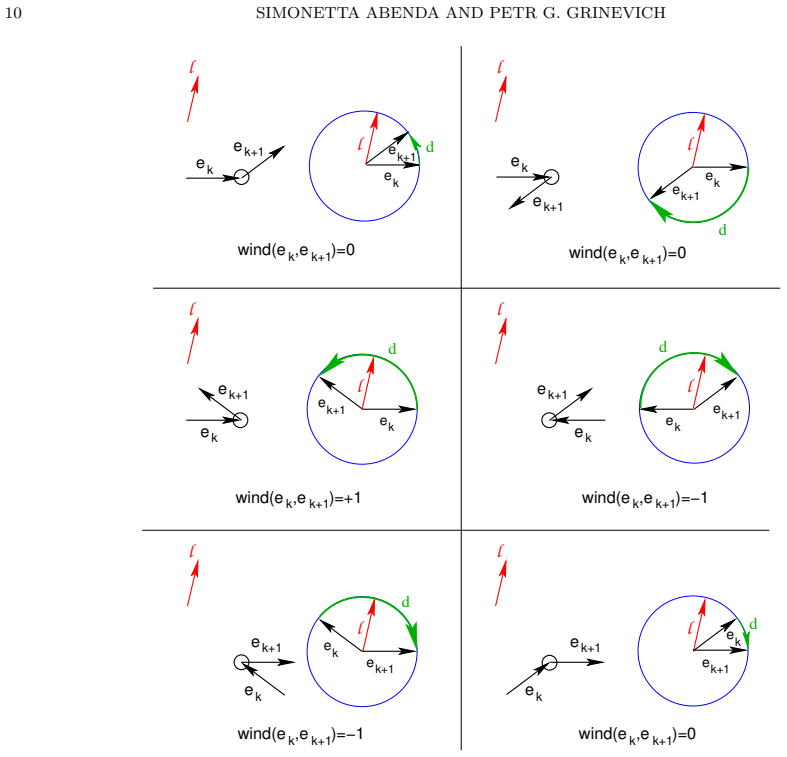
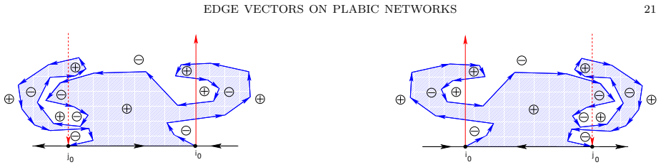
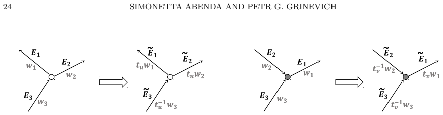
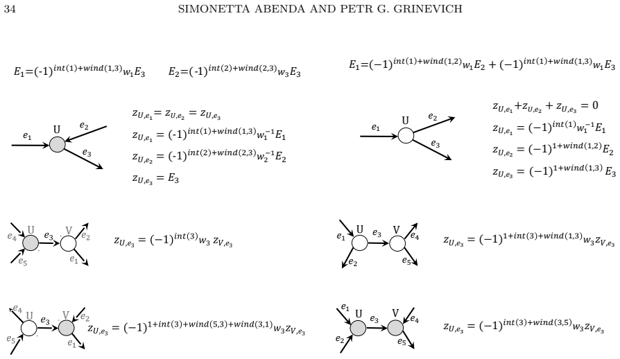
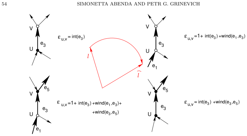
The central object is the geometric signature: a bit $\epsilon_{U,V}$ assigned to each edge of the oriented network, computed from two geometric indices — the local winding number of an ordered pair of edges around a fixed gauge ray direction $l$, and the number of intersections of the edge with gauge rays emitted from the boundary sources. The Lam system writes these bits into relations $z_{U,e}=(-1)^{\epsilon_{U,V}}w_{U,V}z_{V,e}$ at edges, equality at black vertices, and a zero sum at white vertices. The signature carries the whole argument because Theorem 7.16 says it is the only choice, up to gauge equivalence, that guarantees full rank and total non-negativity for all positive weights; its face-level counterpart (Theorem 7.23) says the total signature around any face is just the parity of the number of white vertices on it.
What would settle it
Test the sign obstruction in equation (7.16) on a small PBDTP graph: pick a signature that differs from the geometric one in parity on some boundary-to-boundary path or some conservative cycle, and choose positive weights concentrated on that path or cycle with all other weights of order $\delta \ll 1$. The theorem predicts that some boundary matrix entry, or its denominator, changes sign and breaks total non-negativity for sufficiently small $\delta$; finding a non-geometric signature whose matrix stays totally non-negative for all positive weights on such a graph would disprove Theorem 7.16.
Extended reading notes
Core claim
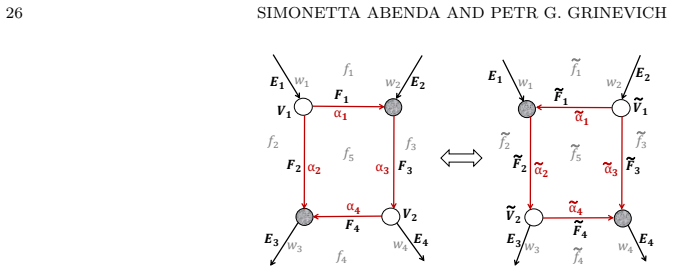
The central claim, Theorem 7.16, is a complete characterization. Let $G$ be a PBDTP plabic graph representing an irreducible positroid cell $S^{TNN}_M$. A signature $\epsilon_{U,V}$ on the edges induces a Lam system of relations that has full rank and a totally non-negative image for every choice of positive weights if and only if $\epsilon_{U,V}$ is equivalent to the geometric signature; in that case the boundary-source solution is exactly the Postnikov boundary measurement matrix and the image is $S^{TNN}_M$. The geometric signature is unique up to gauge equivalence, and the paper shows that changes of orientation, gauge-ray direction, and vertex position act as gauge transformations of the signature. The paper also gives rational formulas for the edge-vector components at internal edges, extending Talaska's flow formula to the interior of the graph.
Load-bearing premise
The load-bearing premise is the PBDTP condition: every edge of the plabic graph must lie on at least one directed path from the boundary back to the boundary; if any edge fails this, path and cycle parities no longer determine a signature and the 'if and only if' statement gains extra gauge freedom.
Editorial extensions
If this is right
- Lam's program for plabic networks in the disk is settled: the signatures that preserve total non-negativity under amalgamation of $\mathrm{Gr}^{TP}(1,3)$ and $\mathrm{Gr}^{TP}(2,3)$ are precisely the geometric ones.
- The boundary measurement matrix is recovered as the unique solution of the geometric linear system at boundary sources, so internal edge vectors give a consistent extension of Postnikov's and Talaska's boundary formulas into the graph.
- On acyclically orientable graphs, all edge-vector components are subtraction-free rational functions of the positive weights, and null edge vectors cannot occur.
- For graphs that are not PBDTP, the completeness statement must be modified; the extra gauge freedom at edges not lying on boundary-to-boundary paths is untrivial and can even support null edge vectors on reducible networks.
- The face-level signature formula connects the geometric signature to Kasteleyn and dimer sign conditions, and the paper identifies its master signature on Le-networks as geometric.
Reading between the lines
- If Theorem 7.16 is right, it gives a practical criterion: to test whether a proposed relation system on a disk plabic network is admissible, one only needs to compare path and cycle parities with the geometric signature, avoiding direct checks over all positive weights.
- The PBDTP condition may be the right generality for a slightly weaker statement: without it, signatures are still constrained on boundary-to-boundary paths and cycles, but the leftover edge gauge degrees of freedom likely form a finite-dimensional family; classifying that family would extend the theorem to arbitrary plabic graphs.
- The face-signature formula suggests a direct bridge to dimer models: one could try to realize the geometric signature explicitly as a Kasteleyn sign matrix on any PBDTP graph, not only on reduced bipartite graphs, and use it to count perfect matchings with boundary conditions.
- A natural testable extension, mentioned as an open problem in the paper, is the same construction on networks in the annulus or on other surfaces with boundary; the gauge-ray machinery should adapt with a modified Talaska formula, but the signature classification may pick up new topological invariants.
Signed reviews
Editorial analysis
A structured set of objections, weighed in public.
Referee Report
Summary. The paper develops a theory of edge vectors on planar bicolored directed trivalent perfect (plabic) networks in the disk that parametrize totally non-negative positroid cells. The central construction assigns to each edge a vector whose components are signed sums over directed paths from that edge to boundary sinks, with signs determined by a winding index relative to a gauge ray direction and by intersections with gauge rays. The authors prove that the resulting vertex relations have full rank (Theorem 3.11), that the edge-vector components are rational functions of the weights with subtraction-free denominators and explicit flow expansions (Theorem 3.12), and that the edge vectors transform predictably under changes of orientation, gauge ray direction, vertex and weight gauge, and Postnikov moves. In Section 7 the vertex relations are recast as Lam's half-edge relations, and geometric signatures are introduced. The main completeness result, Theorem 7.16, states that for a PBDTP graph representing an irreducible positroid cell, a signature gives a full-rank system with totally non-negative image for every choice of positive weights if and only if it is equivalent to the geometric signature, in which case the boundary solution is the Postnikov boundary measurement matrix and the image is the expected positroid cell. The paper also gives a face formula for geometric signatures and an interpretation of the relations as totally non-negative amalgamation of small Grassmannians.
Significance. If Theorem 7.16 is correct, it answers Lam's signature question for the PBDTP subclass of plabic networks and gives a concrete bridge among geometric relations, boundary measurement matrices, and amalgamation of totally non-negative Grassmannians. The paper's strengths are its explicit and constructive character: the full-rank statement in Theorem 3.11 is proved by identifying the determinant with the sum of conservative-flow weights, the edge-vector components are given by closed Talaska-type flow formulas, and the invariance and vertex-consistency checks are carried out in the appendices. The main caveat is that the advertised completeness is proved only under the PBDTP hypothesis, and the relation between this hypothesis and the stated claim of completeness needs to be made precise in the published version.
major comments (3)
- [Definition 2.5; Lemma 7.14; Remark 7.15; Theorem 7.16] The completeness theorem is proved only for PBDTP graphs, and the PBDTP condition is load-bearing in Lemma 7.14: the step in which equal parities on all boundary-to-boundary paths and cycles are converted into gauge equivalence of signatures uses the fact that every edge lies on such a path. Remark 7.15 explicitly concedes that outside this class there is extra gauge freedom and that the statement of Theorem 7.16 must be modified. The abstract and the introduction nevertheless advertise a 'complete and explicit characterization' and describe the setting as 'optimal.' Since the paper gives no concrete non-PBDTP graph for which a non-geometric signature still has full rank and totally non-negative image for all positive weights, it does not establish that PBDTP is the optimal domain. The authors should either provide such an example or an argument that none exists, or rephrase the advertised completeness claim as a characterization on the PBDTP subclass.
- [Abstract; Section 7.3 (Remark 7.24, Conjecture 7.25)] The abstract states that 'the image of the boundary measurement map and the dimer partition functions do not coincide if the graph is not bipartite.' I could not find this assertion stated or proved anywhere in the body. Section 7.3 only conjectures a Kasteleyn-type interpretation for PBDTP graphs and notes that for reduced bipartite graphs the geometric signature realizes Speyer's variant; no non-bipartite comparison is proved. This claim should be removed from the abstract or supported by a proof in the text.
- [Theorem 7.16, Step 3 (Eqs. (7.18)–(7.19))] The asymptotic sign argument in Step 3 of the proof of Theorem 7.16 draws conclusions about the sign of the matrix entry A_{ij} from total non-negativity. Total non-negativity is a condition on maximal minors, not directly on individual entries of the reduced row echelon form. The argument should explicitly use the fixed-sign relation between A_{ij} and the maximal minor obtained by replacing the pivot column i_r with column j, or else state the sign convention that makes this implication immediate. This is a local proof gap rather than an error in the statement, but it is part of the proof of the central theorem and should be repaired.
minor comments (4)
- [Abstract and Section 1] The phrase 'complete and explicit characterization' appears before the PBDTP hypothesis is introduced; state the hypothesis at the first mention of completeness so that the scope of the theorem is visible to the reader.
- [Section 1] The word 'optimal' in the description of the PBDTP setting is stronger than what is proved. Replacing it with 'the setting in which we prove completeness' would better match the content of Theorem 7.16 and Remark 7.15.
- [Example 3.15 and Section 6] Example 3.15 gives a clear demonstration that null edge vectors can occur on reducible networks. It would help the reader if the example were referenced again at the beginning of Section 6, where the phenomenon is discussed systematically.
- [Definition 3.4 and Eq. (3.5)] The notation int(e) in Eq. (3.5) refers to the edge incident to a boundary sink, but the same symbol is used earlier for the intersection number of an arbitrary edge in a path. Clarify that the boundary edge has its own intersection number, since the distinction is used in several later formulas.
Circularity Check
No significant circularity: the completeness theorem is proven from Postnikov and Talaska benchmarks, with the PBDTP restriction explicitly flagged as a limitation rather than smuggled in.
full rationale
The paper's central claim, Theorem 7.16, is an if-and-only-if statement: a signature on a PBDTP graph yields full-rank Lam relations with totally non-negative image for all positive weights exactly when it is equivalent to the geometric signature. The forward direction follows from Theorem 7.7, which re-expresses the previously constructed edge-vector system in Lam form and identifies the boundary solution with the Postnikov boundary measurement matrix; this uses external results of Postnikov and Talaska as benchmarks. The reverse direction is proved directly in Steps 1-4 of Theorem 7.16: after the sign-weight substitution (7.14), the Talaska-type formula (7.16) is used to show that total non-negativity forces the parity of the signature on every boundary-to-boundary path and every one-component conservative flow to match the geometric signature, and then Lemma 7.14 converts this parity coincidence into gauge equivalence. The key reduction (7.18) and (7.19) is a path-weight dominance argument, not an assumption of the conclusion. The PBDTP hypothesis is expressly stated as essential in Remark 7.15: edges not on any boundary-to-boundary path never enter the boundary measurement and admit extra gauge freedom, so the theorem is honestly scoped rather than circular. The paper does contain self-citations, notably to the authors' prior work [4] for the master signature on Le-networks, but that citation is not load-bearing for the completeness proof: the same section gives a direct construction by drawing gauge rays almost horizontally so that the master signature coincides with the geometric signature. One non-circular defect is that the abstract claims that boundary-measurement images and dimer partition functions do not coincide for non-bipartite graphs, while the body does not appear to provide a proof or location for this claim; this is a missing-support/correctness issue, not a circularity issue.
Assumptions & free parameters
assumptions (5)
- domain assumption Graphs are planar bicolored directed trivalent perfect graphs in the disk with boundary vertices on a common interval and each boundary edge attached to an internal bivalent white vertex (Definition 2.3, Remark 2.4).
- domain assumption PBDTP condition: every edge belongs to at least one directed path from boundary to boundary (Definition 2.5).
- domain assumption The gauge ray direction l is generic: no internal edge is parallel to l and no boundary gauge ray passes through an internal vertex (Definition 3.1).
- domain assumption Edge weights are positive real numbers, and for acyclically orientable networks they are expressed in a canonical basis.
- standard math Background results from Postnikov's boundary measurement map, Talaska's flow formula for Plücker coordinates, and Lam's amalgamation framework are taken as established.
Cite this review
Pith. "Pith review of Edge vectors on plabic networks in the disk and amalgamation of totally non-negative Grassmannians." pith.science (2026). https://pith.science/paper/IEZ7QYFJ
@misc{pith2026190807437,
  author       = {Pith},
  title        = {Pith review of: Edge vectors on plabic networks in the disk and amalgamation of totally non-negative Grassmannians},
  year         = {2026},
  howpublished = {\url{https://pith.science/paper/IEZ7QYFJ}},
  note         = {Machine review of arXiv:1908.07437}
}
abstract
Amalgamation in the totally non-negative part of positroid varieties is equivalent to gluing copies of $Gr^{TP}(1,3)$ and $Gr^{TP}(2,3)$. Lam has proposed to represent amalgamation in positroid varieties by equivalence classes of relations on bipartite graphs and identify total non-negativity via edge signatures. Here we provide an explicit characterization of such signatures on the planar bicolored trivalent directed perfect networks in the disk parametrizing positroid cells $S_M^{TNN}$.To a graph $G$ representing $S_M^{TNN}$, we associate a geometric signature satisfying full rank condition and total non--negativity. Such signature is uniquely identified by geometric indices ruled by orientation and gauge ray direction. The image of this map coincides with that of Postnikov boundary measurement map. We solve the system of geometric relations generalizing Postnikov's and Talaska's results for the boundary edges to the internal edges of the graphs: the edge vector components are rational in the weights with subtraction--free denominators, and have explicit expressions in terms of conservative and edge flows. At boundary sources the edge vectors give the boundary measurement matrix. If $G$ is acyclically orientable, all components are subtraction-free rational in the weights w.r.t. a convenient basis. We provide explicit formulas for the transformation rules w.r.t. changes the orientation, the several gauges of the given network, moves and reductions of networks. We show that the image of the boundary measurement map and the dimer partition functions do not coincide if the graph is not bipartite.
Figures


Figures from the paper (33 more)













Reference graph
Works this paper leans on
-
[7]
Vector-relation configurations and plabic graphs
Affolter, N., M. Glick, P. Pylyavskyy, and S. Ramassamy, Vector–relation configurations and plabic graphs arXiv1908.06959v1
-
[1]
Kasteleyn theorem, geometric signatures and KP-II divisors on planar bipartite networks in the disk
S. Abenda, Kasteleyn theorem, geometric signatures and KP-II divisors on planar bipartite networks in the disk, arXiv:2012.13797
work page Pith review arXiv 2012
-
[2]
Rational degenerations of M-curves, totally positive Grassmannians and KP–solitons
Abenda, S., and P.G. Grinevich, “Rational degenerations of M-curves, totally positive Grassmannians and KP–solitons.” Commun. Math. Phys. 361, no. 3 (2018): 1029–1081
work page 2018
-
[3]
Abenda, S., and P.G. Grinevich, “Real soliton lattices of the Kadomtsev-Petviashvili II equation and desin- gularization of spectral curves corresponding to GrTP(2, 4).” Proc. Steklov Inst. Math. 302, no. 1 (2018): 1–15
work page 2018
-
[4]
Abenda, S., and P.G. Grinevich, “Reducible M-curves for Le-networks in the totally-nonnegative Grassmannian and KP–II multiline solitons.” Sel. Math. New Ser. 25, no. 3 (2019) 25:43. https://doi.org/10.1007/s00029-019-0488-5
-
[5]
KP theory, plabic networks in the disk and rational degenerations of M--curves
Abenda, S., and P.G. Grinevich, KP theory, plabic networks in the disk and rational degenerations of M–curves. arXiv:1801.00208
-
[6]
Abenda, S., and P.G. Grinevich, Amalgamation in totally non-negative Grassmannians and real regular KP divisors on M–curves., in prep. (2019)
work page 2019
-
[8]
Arkani–Hamed, N., J.L. Bourjaily, F. Cachazo, A.B. Goncharov, A. Postnikov, and J. Trnka, Scattering Amplitudes and the Positive Grassmannian. , arXiv:1212.5605. 58 SIMONETTA ABENDA AND PETR G. GRINEVICH
Show all 58 references
-
[9]
Bourjaily, F
Arkani–Hamed, N., J.L. Bourjaily, F. Cachazo, A.B. Goncharov, A. Postnikov, and J. Trnka, Grassmannian geometry of scattering amplitudes. Cambridge University Press, Cambridge, 2016
2016
-
[10]
Twistor theory at fifty: from contour integrals to twistor strings
Atiyah, M., M. Dunajski, and L.J. Mason, “Twistor theory at fifty: from contour integrals to twistor strings.” Proc. R. Soc. A. 473 (2017): 20170530, 33 pp
2017
-
[11]
Suris, Discrete differential geometry
Bobenko, A.I., and Y.B. Suris, Discrete differential geometry. Integrable structure. Graduate Studies in Math- ematics, 98, Amer.Mathem.Soc., Providence, RI, 2008. xxiv+404 pp
2008
-
[12]
Stratifying on–shell cluster varieties: the geometry of non–planar on–shell diagrams
Bourjaily, J.L., S. Franco, D. Galloni, and C. Wen, “Stratifying on–shell cluster varieties: the geometry of non–planar on–shell diagrams.” J. High Energy Phys. (2016), no. 10, 003, front matter+30 pp
2016
-
[13]
Glutsyuk, Total positivity, Grassmannian and modified Bessel functions
Buchstaber, V., and A. Glutsyuk, Total positivity, Grassmannian and modified Bessel functions. arXiv:1708.02154
-
[14]
Soliton solutions of the KP equation and application to shallow water waves
Chakravarty, S., and Y. Kodama, “Soliton solutions of the KP equation and application to shallow water waves.” Stud. Appl. Math. 123 (2009): 83–151
2009
-
[15]
Tableaux combinatorics for the asymmetric exclusion process
Corteel, S., and L.K. Williams, “Tableaux combinatorics for the asymmetric exclusion process.” Adv. in Appl. Math. 39, no. 3 (2007): 293–310
2007
-
[16]
Multidimensional quadrilateral lattices are integrable
Doliwa, A., and P.M. Santini, “Multidimensional quadrilateral lattices are integrable.” Phys. Lett. A 233, no 4–6 (1997): 365–372
1997
-
[17]
Real theta-function solutions of the Kadomtsev-Petviashvili equation
Dubrovin, B. A., and S.M. Natanzon, “Real theta-function solutions of the Kadomtsev-Petviashvili equation.” Izv. Akad. Nauk SSSR Ser. Mat. 52 (1988): 267–286
1988
-
[18]
Cluster X –Varieties, Amalgamation and Poisson-Lie Groups
Fock, V.V., and A. B. Goncharov, “Cluster X –Varieties, Amalgamation and Poisson-Lie Groups.”, in Al- gebraic Geometry and Number Theory, dedicated to Drinfeld’s 50th birthday, pp. 27–68, Progr. Math. 253, Birkhauser, Boston, 2006
2006
-
[19]
Loop–erased walks and total positivity
Fomin, S., “Loop–erased walks and total positivity.” Trans. of the AMS 353, no. 9 (2001): 3563–3583
2001
-
[20]
Pylyavskyy, and E
Fomin, S., P. Pylyavskyy, and E. Shustin, Morsifications and mutations. arXiv:1711.10598 (2017)
2017 arXiv
-
[21]
Double Bruhat cells and total positivity
Fomin, S., and A. Zelevinsky, “Double Bruhat cells and total positivity.” J. Amer. Math. Soc. 12 (1999): 335–380
1999
-
[22]
Cluster algebras I: foundations
Fomin S., and A. Zelevinsky, “Cluster algebras I: foundations.” J. Am. Math. Soc. 15 (2002): 497–529
2002
-
[23]
The totally nonnegative Grassmannian is a ball
Galashin, P., S.N. Karp, and T. Lam, “The totally nonnegative Grassmannian is a ball.” S´ eminaire Lotharingien de Combinatoire 80B (2018): Article #23, 12 pp
2018
-
[24]
Sur les matrices oscillatoires
Gantmacher, F.R., and M.G. Krein, “Sur les matrices oscillatoires.” C.R. Acad. Sci. Paris 201 (1935): 577– 579
1935
-
[25]
Krein, Oscillation Matrices and Kernels and Small Vibrations of Mechanical Systems
Gantmacher, F.R., and M.G. Krein, Oscillation Matrices and Kernels and Small Vibrations of Mechanical Systems. (Russian), Gostekhizdat, Moscow- Leningrad, (1941), second edition (1950), English edition from AMS Chelsea Publ. (2002)
1941
-
[26]
Poisson geometry of directed networks in a disk
Gekhtman, M., M. Shapiro, and A. Vainshtein, “Poisson geometry of directed networks in a disk”, Selecta Math. 15 (2009): 61–103
2009
-
[27]
Shapiro, and A
Gekhtman, M., M. Shapiro, and A. Vainshtein, Cluster algebras and Poisson geometry. Mathematical Surveys and Monographs, 167. American Mathematical Society, Providence, RI, (2010), xvi+246 pp
2010
-
[28]
Poisson Geometry of Directed Networks in an Annulus
Gekhtman M., M. Shapiro, and A. Vainshtein, “Poisson Geometry of Directed Networks in an Annulus.” J. of the Europ. Math. Soc. 14 (2012): 541–570
2012
-
[29]
Combinatorial geometries, convex polyhedra, and Schubert cells
Gel’fand, I.M., R.M. Goresky, R.D. MacPherson, and V.V. Serganova, “Combinatorial geometries, convex polyhedra, and Schubert cells.” Adv. in Math. 63, no. 3 (1987): 301–316
1987
-
[30]
Combinatorial geometries and torus strata on homogeneous compact manifolds
Gel’fand, I.M., and V.V. Serganova, “Combinatorial geometries and torus strata on homogeneous compact manifolds.” Russian Mathematical Surveys 42, no. 2 (1987): 133–168
1987
-
[31]
Dimers and cluster integrable systems
Goncharov, A.B., and R. Kenyon, “Dimers and cluster integrable systems.” Ann. Sci. ´Ec. Norm. Sup´ er.(4) 46, no. 5 (2013): 747–813
2013
-
[32]
Unraveling Ln;k Grassmannian Kinematics
Kaplan, J., “Unraveling Ln;k Grassmannian Kinematics.” J. High Energy Phys. 2010, no. 3, 025, (2010) 34 pp
2010
-
[33]
Karlin, S., Total Positivity, Vol. 1. Stanford, 1968
1968
-
[34]
Kasteleyn, The statistics of dimers on a lattice.I
P.W. Kasteleyn, The statistics of dimers on a lattice.I. The number of dimer arrangements on a quadratics lattice, Physica 27 (1961), 1209-1225
1961
-
[35]
Kasteleyn, Graph theory and crystal physics, in Graph Theory and Theoretical Physics , Ed
P. Kasteleyn, Graph theory and crystal physics, in Graph Theory and Theoretical Physics , Ed. F. Harary, Academic Press, London (1967) pp. 43-110
1967
-
[36]
Planar dimers and Harnack curves
Kenyon, R., and A. Okounkov, “Planar dimers and Harnack curves.” Duke Math. J. 131, no. 3 (2006): 499– 524
2006
-
[37]
The Deodhar decomposition of the Grassmannian and the regularity of KP solitons
Kodama, Y. and L.K. Williams, “The Deodhar decomposition of the Grassmannian and the regularity of KP solitons.” Adv. Math. 244 (2013): 979–1032. EDGE VECTORS ON PLABIC NETWORKS 59
2013
-
[38]
KP solitons and total positivity for the Grassmannian
Kodama, Y. and L.K. Williams, “KP solitons and total positivity for the Grassmannian.” Invent. Math. 198 (2014) 637–699
2014
-
[39]
Spectral theory of two-dimensional periodic operators and its applications
Krichever, I.M., “Spectral theory of two-dimensional periodic operators and its applications”, Russian Math. Surveys, 44, no. 8 (1989): 146–225
1989
-
[40]
Dimers, webs, and positroids
Lam, T., “Dimers, webs, and positroids.”, J. Lond. Math. Soc. (2) 92, no. 3 (2015): 633–656
2015
-
[41]
Press, Somerville, MA, 2016
Lam, T., Totally nonnegative Grassmannian and Grassmann polytopes., Current developments in mathematics 2014, 51–152, Int. Press, Somerville, MA, 2016
2014
-
[42]
Birkh¨ auser, 1991
Lawler, G., Intersections of random walks. Birkh¨ auser, 1991
1991
-
[43]
Total positivity in reductive groups
Lusztig, G., “Total positivity in reductive groups.” Lie Theory and Geometry: in honor of B. Kostant , Progress in Mathematics 123, Birkh¨ auser, Boston, 1994, 531–568
1994
-
[44]
Total positivity in partial flag manifolds
Lusztig, G., “Total positivity in partial flag manifolds.” Representation Theory 2 (1998), 70–78
1998
-
[45]
Parametrizations of flag varieties
Marsh, R. J. and K. Rietsch, “Parametrizations of flag varieties.” Represent. Theory 8 (2004): 212–242
2004
-
[46]
Dual Superconformal Invariance, Momentum Twistors and Grassmannians
Mason, L., and D. Skinner, “Dual Superconformal Invariance, Momentum Twistors and Grassmannians.” J. High Energy Phys. 2009, no. 11, 045, (2009), 39 pp
2009
-
[47]
Weak separation and plabic graphs
Oh, S., A. Postnikov, and D.E. Speyer, “Weak separation and plabic graphs.” Proc. Lond. Math. Soc. (3) 110, no. 3 (2015): 3, 721–754
2015
-
[48]
, arXiv:math/0609764 [math.CO]
Postnikov, A., Total positivity, Grassmannians, and networks. , arXiv:math/0609764 [math.CO]
-
[49]
, arXiv:1806:05307
Postnikov, A., Positive Grassmannian and polyhedral subdivisions. , arXiv:1806:05307
-
[50]
Matching polytopes, toric geometry, and the totally non-negative Grassmannian
Postnikov, A., D. Speyer, and L. Williams, “Matching polytopes, toric geometry, and the totally non-negative Grassmannian.” J. Algebraic Combin. 30, no. 2 (2009): 173–191
2009
-
[51]
An algebraic cell decomposition of the nonnegative part of a flag variety
Rietsch, K., “An algebraic cell decomposition of the nonnegative part of a flag variety.” Journal of Algebra 213, no. 1 (1999): 144–154
1999
-
[52]
The totally nonnegative part of G/P is a CW complex-
Rietsch, K., and L. Williams, “The totally nonnegative part of G/P is a CW complex-”, Transform. Groups 13, no- 3–4 (2008): 839–853
2008
-
[53]
¨Uber variationsvermindende lineare Transformationen
Schoenberg, I., “ ¨Uber variationsvermindende lineare Transformationen.” Math. Zeit. 32, (1930): 321–328
1930
-
[54]
Grassmannians and cluster algebras
Scott J.S., “Grassmannians and cluster algebras.” Proc. London Math. Soc. 92 (2006): 345–380
2006
-
[55]
The pentagram map
Schwartz, R. “The pentagram map.”, Experiment. Math. 1, no. 1 (1992): 71–81
1992
-
[56]
Variations on a theme of Kasteleyn, with application to the totally nonnegative Grassmannian
Speyer, D.E. “Variations on a theme of Kasteleyn, with application to the totally nonnegative Grassmannian.” Electron. J. Combin. 23, no. 2 (2016) Paper 2.24, 7 pp
2016
-
[57]
A Formula for Pl¨ ucker Coordinates Associated with a Planar Network
Talaska, K., “A Formula for Pl¨ ucker Coordinates Associated with a Planar Network.” IMRN 2008, (2008), Article ID rnn081, 19 pages
2008
-
[58]
Network parametrizations for the Grassmannian
Talaska, K., and L. Williams, “Network parametrizations for the Grassmannian.” Alg. Numb. Th. 7, no. 9 (2013): 2275–2311. Dipartimento di Matematica and Alma Mater Research Center on Applied Mathematics, Univer- sit`a di Bologna, Italy, INFN, sez. di Bologna, Italy Email addre...
2013
Reviewed August 14, 2026 · model on record in the stance chip above.
Discussion (0). Continue with ORCID to comment.