REVIEW 3 major objections 6 minor 1 cited by
A comparison between solar plage and network properties
T0 review · 3 major / 6 minor · reviewed 2026-08-14 · deepseek-v4-flash
Pith's one-line read The paper shows that kilogauss magnetic patches in the solar network are intrinsically stronger, brighter, and surrounded by faster downflows than equally sized patches in plage.
desk verdict A careful, size-resolved comparison showing network kG patches are intrinsically different from plage patches of the same size, with the main caveat that environment-dependent inversion bias is not fully excluded. read the letter →
The pith
A machine-rendered reading of the paper's core claim, the machinery that carries it, and where it could break.
The reading
What carries the argument
The central object is the size-matched kG patch: a connected region of pixels with $B>1$ kG at $\log\tau = -0.8$, binned by area before comparison so that network and plage patches of equal size can be compared directly. The properties themselves come from the 2D SPINOR inversion of the Fe I 6302 Å line pair, a spatially coupled inversion that assigns one model atmosphere per pixel and compensates for the telescope point-spread function, removing the need for a stray-light component. The size binning is the mechanism that isolates intrinsic differences from the differing patch size distributions of the two environments.
What would settle it
Re-observe the same network and plage regions at a spatial sampling finer than 0.1 arcsec, or run the same 2D inversion on synthetic spectra from magnetohydrodynamic simulations of network and plage, and repeat the size-matched comparison; if the 150 G, 5%, and 800 m/s differences shrink or vanish once the smallest patches are fully resolved, the reported offsets are resolution or inversion artifacts rather than intrinsic environment effects.
Extended reading notes
Core claim
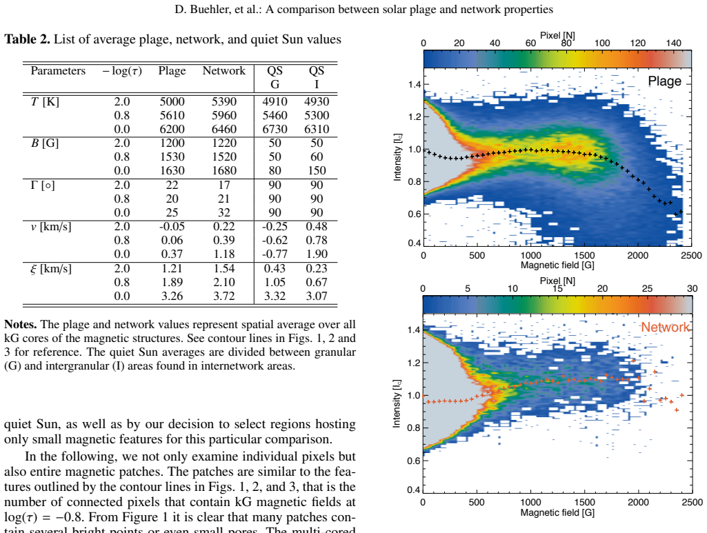
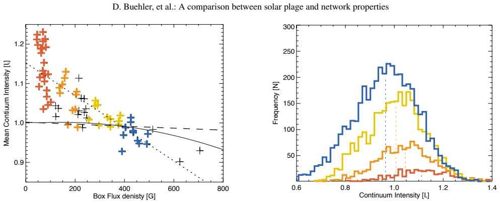
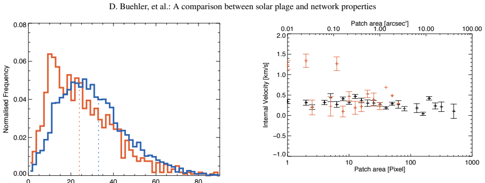
At $\log\tau = -0.8$, individual kilogauss patches are defined as connected pixels with fields above 1 kG and then binned by area. In every size bin, network patches have mean field strengths about 150 G higher than equally sized plage patches and continuum contrasts about 5% higher; at disc centre the typical network patch is about 10% brighter than the mean quiet Sun while the typical plage patch is about 3% darker. The one-pixel ring around each network patch hosts downflows at $\log\tau = 0$ averaging 800 m/s faster than the ring around an equally sized plage patch, and the downflow speed grows with patch area so that average maximum downflows exceed 11 km/s around the largest pore-containing plage patches. Plage canopies are on average 9 degrees more horizontal than network canopies. The paper interprets the size-matched residuals as evidence that the convective environment, not the patch size alone, sets the field strength and brightness of these small magnetic elements.
Load-bearing premise
The comparison assumes that the 2D inversion recovers the true field strength, continuum intensity, and velocity of small kilogauss patches equally well in the network and in the plage, with no size- or environment-dependent bias at 0.16 arcsec sampling; the paper itself notes residual scattered light and that the smallest kG features are not completely resolved.
Editorial extensions
If this is right
- Irradiance reconstructions that assign brightness from patch size alone will miss the ~5% environment-dependent contrast offset, so area-based models need a network/plage correction term.
- MHD and thin-flux-tube models of small magnetic elements must reproduce stronger, brighter network patches with faster surrounding downflows at the same size, constraining convective-collapse and heating mechanisms.
- The growth of surrounding downflow speed with patch area, up to supersonic values near pores, unifies bright points and pores on a single scaling relation for the energy available to drive photospheric and chromospheric flows.
- The more horizontal plage canopy offers a structural reason for the different chromospheric organisation above active regions, such as the preponderance of spicules there, which can be tested against chromospheric observations.
Reading between the lines
- A direct extension would be to bin the existing data by local flux density rather than by network/plage label; if the size-matched offsets are caused by modified convection, they should appear within a single region type as the ambient flux density rises.
- If the 800 m/s downflow gap persists at full resolution, the environment-dependent kinetic energy flux from downflow rings could be fed into models of p-mode absorption or spicule driving, a step the paper does not take.
- Applying the same patch-binning recipe to spectropolarimetric data of an emerging flux region would test whether plage-like patch properties arise from flux density alone or from the presence of sunspots and pores.
Signed reviews
Editorial analysis
A structured set of objections, weighed in public.
Referee Report
Summary. This paper compares kG magnetic structures in solar network and plage using six Hinode SP scans near disc centre, inverted with the 2D SPINOR code. The authors identify connected patches of kG field at log(τ) = -0.8 and compare patch size, mean field strength, continuum intensity, internal and surrounding LOS velocities, inclination, and microturbulence. The headline result is a size-matched comparison: at equal patch area, network features are on average ~150 G stronger, ~5% brighter in continuum, and surrounded by ~800 m/s faster downflows than plage features, while the overall mean field strength of kG pixels is ~1.5 kG in both. The paper concludes that most network-plage differences reflect different patch-size distributions, but that a residual intrinsic difference likely results from modified convection in flux-rich plage.
Significance. If correct, the size-matched differences overturn the classical picture that network and plage magnetic elements are intrinsically identical except for size distribution. The paper's methodology is stronger than earlier low-resolution comparisons: it uses seeing-free SP data, a spatially coupled 2D inversion with one atmosphere per pixel, and multiple cross-checks (exposure-time consistency, sub-FOV flux-density matching, comparison of noise levels). These strengths make the comparison internally consistent. The central risk is that the 2D inversion itself may introduce size- or environment-dependent biases, which the paper acknowledges but does not quantify; a synthetic MHD test would resolve this.
major comments (3)
- [Section 3 (Fig. 6) and Section 4] The central claim that network and plage kG features differ intrinsically at equal patch size requires that the 2D SPINOR inversion recovers intrinsic field strength, continuum intensity, and velocity without size- or environment-dependent bias. The manuscript itself provides evidence that this condition is not fully met: Figure 6 shows an rms continuum contrast of 11.8% versus 14.4% in MHD simulations, and Section 4 states that the smallest kG features are not completely resolved. Because SPINOR is spatially coupled and the patch-selection threshold B ≥ 1 kG can behave differently in dense plage than in sparse network, the size-matched B and I differences could be generated by inversion systematics. I request a synthetic test: degrade MHD snapshots (e.g., MuRAM) to SP resolution and noise, invert with the same SPINOR setup and patch-selection pipeline, and verify that the recovered network-versus-plage differences are unbiased. This test is needed before the 150 G and 5% results can be considered robust.
- [Section 3.3, Figs. 16-17] The one-pixel-wide ring used to measure surrounding downflows is narrower than the SP point-spread function (0.16 arcsec pixels, diffraction limit near 0.3 arcsec). Ring and patch pixels are therefore not independent after the deconvolution inherent in 2D SPINOR. The 800 m/s network-plage offset in ring velocity at equal patch area could reflect different PSF cross-talk between isolated network features and crowded plage features. Please test robustness to ring width (e.g., 2-3 pixels) and to PSF assumptions; this bears directly on the headline downflow claim.
- [Section 3.1, Fig. 10; Abstract; Section 5] The manuscript gives inconsistent values for a headline quantity: the text near Figure 10 states that network fields are ~100 G stronger than plage fields for any given patch area, whereas the Abstract and Section 5 state 150 G. Additionally, the binned means in Figures 9, 10, and 16 are presented with only the error of the mean, without a significance test on the difference or sample sizes per bin. Please reconcile the numbers and add significance estimates (e.g., bootstrap confidence intervals on the differences) for the three headline quantities: 150 G, 5%, and 800 m/s.
minor comments (6)
- [Abstract] The phrase "the modification of the convection photospheric convection" should be "the modification of photospheric convection"; the abstract also contains the grammatical error "is likely results from".
- [Section 5] The first sentence of the conclusion contains the typo "A more detailled inspection" for "detailed".
- [Table 2] The caption labels the quiet Sun columns as "QS G I", which is unclear; please expand to "quiet Sun granular" and "quiet Sun intergranular" and explain why two quiet Sun columns are needed.
- [Figures 5 and 7] The text references "coloured crosses" and a colour scheme that is identical to Figure 5, but the caption does not define the colour mapping; a legend or explicit description would help the reader.
- [Section 5] The claim that the maximum downflows exceed 11 km/s, "faster than any previously reported photospheric flow outside of a sunspot", lacks an explicit citation and should be quantified or qualified.
- [Figures 9 and 10] The horizontal axis is labelled "Patch size [Pixel]" in Figure 9 and "Patch area [Pixel]" in Figure 10; please use consistent terminology for patch area.
Circularity Check
No significant circularity: the size-matched network–plage differences are direct comparisons of inverted Hinode data, not constructions from fitted inputs or self-cited results.
full rationale
The central claims—150 G stronger fields, 5% higher continuum contrast, and 800 m/s faster surrounding downflows for similarly sized network patches—are direct, size-binned comparisons of quantities returned by the SPINOR inversion (Figures 9, 10, 16, and 17). No parameter was fitted to the network/plage labels, and no equation defining one claimed quantity in terms of the other appears in the derivation chain. The inversion uses the same three-node atmosphere for both populations; any residual bias from underresolution or scattered light is a systematic-error concern, not a construction that forces the reported offset. The paper's self-citations (e.g., van Noort 2012 for the 2D inversion and Buehler et al. 2015 for ambiguity resolution) provide methods that are applied symmetrically to plage and network data and do not encode the size-matched differences in advance. Moreover, the paper reproduces the earlier contrary result of Stenflo & Harvey (1985) when canopy fields are included, demonstrating that the analysis is not rigged to produce its headline comparison. The quoted caveat that the smallest kG features are not completely resolved identifies a plausible systematic limitation, but it is not a circular step. On this basis the paper is self-contained with respect to its stated comparison, and no specific reduction of a prediction to its inputs can be exhibited.
Assumptions & free parameters
free parameters (1)
- LOS velocity zero-point correction =
200 m/s
assumptions (5)
- domain assumption 2D SPINOR inversion with three log(tau) nodes and a single atmosphere per pixel retrieves intrinsic photospheric parameters at 0.16 arcsec sampling.
- domain assumption Radiative transfer and atomic line data used by SPINOR/STOPRO accurately model the 6301/6302 A Fe I lines.
- domain assumption Connected pixels with B >= 1 kG at log(tau)=-0.8 define individual magnetic patches and their immediate one-pixel rings.
- domain assumption The 180-degree ambiguity resolution method of Buehler et al. (2015) gives correct field inclinations.
- domain assumption PLA/NET thin flux tube models and MuRAM-based MHD simulations are suitable benchmarks for the inferred temperature and field stratifications.
Cite this review
Pith. "Pith review of A comparison between solar plage and network properties." pith.science (2026). https://pith.science/paper/33CHYLIY
@misc{pith2026190807464,
  author       = {Pith},
  title        = {Pith review of: A comparison between solar plage and network properties},
  year         = {2026},
  howpublished = {\url{https://pith.science/paper/33CHYLIY}},
  note         = {Machine review of arXiv:1908.07464}
}
read the original abstract
We compare the properties of kG magnetic structures in the solar network and in active region plage at high spatial resolution. Our analysis used six SP scans of the solar disc centre aboard Hinode SOT and inverted the obtained spectra of the photospheric 6302 \AA line pair using the 2D SPINOR code. Photospheric magnetic field concentrations in network and plage areas are on average 1.5 kG strong with inclinations of 10-20 degrees, and have <400 m/s internal and 2-3 km/s external downflows. At the disc centre, the continuum intensity of magnetic field concentrations in the network are on average 10% brighter than the mean quiet Sun, whilst their plage counterparts are 3% darker. A more detailed analysis revealed that all sizes of individual kG patches in the network have 150 G higher field strengths on average, 5% higher continuum contrasts, and 800 m/s faster surrounding downflows than similarly sized patches in the plage. The speed of the surrounding downflows also correlates with the patch area, and patches containing pores can produce supersonic flows exceeding 11 km/s in individual pixels. Furthermore, the magnetic canopies of kG patches are on average 9 degrees more horizontal in the plage compared to the network. Most of the differences between the network and plage are due to their different patch size distributions, but the intrinsic differences between similarly sized patches is likely results from the modification of the convection photospheric convection with increasing amounts of magnetic flux.
Figures


Figures from the paper (10 more)




Forward citations
Cited by 1 Pith paper
-
A method for global inversion of multi-resolution solar data
A Levenberg-Marquardt based global inversion method that applies per-dataset linear degradation operators to jointly invert solar spectra at different spatial resolutions.
Reference graph
Works this paper leans on
-
[1]
R., Schlichenmaier, R., & S ¨utterlin, P
Beck, C., Bellot Rubio, L. R., Schlichenmaier, R., & S ¨utterlin, P. 2007, A&A, 472, 607
2007
-
[2]
E., Rouppe van der V oort, L., & L¨ofdahl, M
Berger, T. E., Rouppe van der V oort, L., & L¨ofdahl, M. 2007, ApJ, 661, 1272
work page 2007
-
[3]
Berger, T. E., Rouppe van der V oort, L. H. M., L¨ofdahl, M. G., et al. 2004, A&A, 428, 613
work page 2004
-
[4]
Berger, T. E. & Title, A. M. 1996, ApJ, 463, 365 12 D. Buehler, et al.: A comparison between solar plage and network properties
work page 1996
-
[5]
Bernasconi, P. N., Keller, C. U., Povel, H. P., & Stenflo, J. O. 1995, A&A, 302, 533
work page 1995
-
[6]
A., M´arquez, I., S´anchez Almeida, J., Cabello, I., & Domingo, V
Bonet, J. A., M´arquez, I., S´anchez Almeida, J., Cabello, I., & Domingo, V . 2008, ApJ, 687, L131
work page 2008
-
[7]
K., & van Noort, M
Buehler, D., Lagg, A., Solanki, S. K., & van Noort, M. 2015, A&A, 576, A27
2015
-
[8]
Buehler, D., Lagg, A., van Noort, M., & Solanki, S. K. 2016, A&A, 589, A31 B¨unte, M., Solanki, S. K., & Steiner, O. 1993, A&A, 268, 736
work page 2016
Show all 81 references
-
[9]
2007, A&A, 474, 261
Cameron, R., Sch¨ussler, M., V¨ogler, A., & Zakharov, V . 2007, A&A, 474, 261
2007
-
[10]
2010, ApJ, 723, 440
Cho, K.-S., Bong, S.-C., Chae, J., Kim, Y .-H., & Park, Y .-D. 2010, ApJ, 723, 440
2010
-
[11]
2013, ApJ, 778, 27
Criscuoli, S. 2013, ApJ, 778, 27
2013
-
[12]
2017, ApJ, 847, 93
Criscuoli, S., Norton, A., & Whitney, T. 2017, ApJ, 847, 93
2017
-
[13]
& Uitenbroek, H
Criscuoli, S. & Uitenbroek, H. 2014, A&A, 562, L1 da Silva Santos, J. M., de la Cruz Rodr ´ıguez, J., & Leenaarts, J. 2018, A&A, 620, A124
2014
-
[14]
2008, A&A, 484, L17
Danilovic, S., Gandorfer, A., Lagg, A., et al. 2008, A&A, 484, L17
2008
-
[15]
H., & Sch¨ussler, M
Danilovic, S., R¨ohrbein, D., Cameron, R. H., & Sch¨ussler, M. 2013, A&A, 550, A118
2013
-
[16]
Defouw, R. J. 1976, ApJ, 209, 266
1976
-
[17]
1984, A&A, 139, 435
Deinzer, W., Hensler, G., Sch¨ussler, M., & Weisshaar, E. 1984, A&A, 139, 435
1984
-
[18]
& Lean, J
Foukal, P. & Lean, J. 1988, ApJ, 328, 347
1988
-
[19]
Frazier, E. N. & Stenflo, J. O. 1972, Sol. Phys., 27, 330
1972
-
[20]
K., Fligge, M., & Bruls, J
Frutiger, C., Solanki, S. K., Fligge, M., & Bruls, J. H. M. J. 2000, A&A, 358, 1109
2000
-
[21]
Grossmann-Doerth, U., Sch¨ussler, M., & Solanki, S. K. 1988, A&A, 206, L37
1988
-
[22]
1978, A&A, 70, 537
Holweger, H., Gehlsen, M., & Ruland, F. 1978, A&A, 70, 537
1978
-
[23]
& Stenflo, J
Howard, R. & Stenflo, J. O. 1972, Sol. Phys., 22, 402
1972
-
[24]
2008, Sol
Ichimoto, K., Lites, B., Elmore, D., et al. 2008, Sol. Phys., 249, 233
2008
-
[25]
2007, A&A, 472, 911
Ishikawa, R., Tsuneta, S., Kitakoshi, Y ., et al. 2007, A&A, 472, 911
2007
-
[26]
K., Feller, A., et al
Jafarzadeh, S., Solanki, S. K., Feller, A., et al. 2013, A&A, 549, A116
2013
-
[27]
K., Lagg, A., et al
Jafarzadeh, S., Solanki, S. K., Lagg, A., et al. 2014, A&A, 569, A105
2014
-
[28]
2016, Research in Astronomy and Astrophysics, 16, 78
Ji, K.-F., Xiong, J.-P., Xiang, Y .-Y ., et al. 2016, Research in Astronomy and Astrophysics, 16, 78
2016
-
[29]
L., & Solanki, S
Kahil, F., Riethm¨uller, T. L., & Solanki, S. K. 2017, ApJS, 229, 12
2017
-
[30]
L., & Solanki, S
Kahil, F., Riethm¨uller, T. L., & Solanki, S. K. 2019, A&A, 621, A78
2019
-
[31]
L., Balasubramaniam, K
Keil, S. L., Balasubramaniam, K. S., Smaldone, L. A., & Reger, B. 1999, ApJ, 510, 422
1999
-
[32]
U., Stenflo, J
Keller, C. U., Stenflo, J. O., Solanki, S. K., Tarbell, T. D., & Title, A. M. 1990, A&A, 236, 250
1990
-
[33]
V ., Collados, M., Solanki, S
Khomenko, E. V ., Collados, M., Solanki, S. K., Lagg, A., & Trujillo Bueno, J. 2003, A&A, 408, 1115 Kn¨olker, M. & Sch¨ussler, M. 1988, A&A, 202, 275
2003
-
[34]
K., & Borrero, J
Kobel, P., Solanki, S. K., & Borrero, J. M. 2011, A&A, 531, A112
2011
-
[35]
K., & Borrero, J
Kobel, P., Solanki, S. K., & Borrero, J. M. 2012, A&A, 542, A96
2012
-
[36]
2007, Sol
Kosugi, T., Matsuzaki, K., Sakao, T., et al. 2007, Sol. Phys., 243, 3
2007
-
[37]
A., Solanki, S
Krivova, N. A., Solanki, S. K., Fligge, M., & Unruh, Y . C. 2003, A&A, 399, L1
2003
-
[38]
K., Riethm¨uller, T
Lagg, A., Solanki, S. K., Riethm¨uller, T. L., et al. 2010, ApJ, 723, L164 Langangen, Ø., Carlsson, M., Rouppe van der V oort, L., & Stein, R. F. 2007, ApJ, 655, 615
2010
-
[39]
K., Topka, K
Lawrence, J. K., Topka, K. P., & Jones, H. P. 1993, J. Geophys. Res., 98, 18911
1993
-
[40]
B., Noyes, R
Leighton, R. B., Noyes, R. W., & Simon, G. W. 1962, ApJ, 135, 474
1962
-
[41]
Lites, B. W. & Ichimoto, K. 2013, Sol. Phys., 283, 601
2013
-
[42]
2018, ApJ, 856, 17 Mart´ınez Pillet, V ., Lites, B
Liu, Y ., Xiang, Y ., Erd´elyi, R., et al. 2018, ApJ, 856, 17 Mart´ınez Pillet, V ., Lites, B. W., & Skumanich, A. 1997, ApJ, 474, 810
2018
-
[43]
2008, ApJ, 677, L145
Nagata, S., Tsuneta, S., Suematsu, Y ., et al. 2008, ApJ, 677, L145
2008
-
[44]
& Scharmer, G
Narayan, G. & Scharmer, G. B. 2010, A&A, 524, A3
2010
-
[45]
K., Domingo, V ., Fligge, M., & Sanahuja, B
Ortiz, A., Solanki, S. K., Domingo, V ., Fligge, M., & Sanahuja, B. 2002, A&A, 388, 1036
2002
-
[46]
L., Rast, M
Peck, C. L., Rast, M. P., Criscuoli, S., & Rempel, M. 2019, ApJ, 870, 89
2019
-
[47]
Proctor, M. R. E. & Weiss, N. O. 1982, Reports on Progress in Physics, 45, 1317
1982
-
[48]
S., Del Toro Iniesta, J
Requerey, I. S., Del Toro Iniesta, J. C., Bellot Rubio, L. R., et al. 2014, ApJ, 789, 6
2014
-
[49]
S., Del Toro Iniesta, J
Requerey, I. S., Del Toro Iniesta, J. C., Bellot Rubio, L. R., et al. 2015, ApJ, 810, 79 Riethm¨uller, T. L. & Solanki, S. K. 2017, A&A, 598, A123 Riethm¨uller, T. L. & Solanki, S. K. 2018, arXiv e-prints Riethm¨uller, T. L., Solanki, S. K., Berdyugina, S. V ., et al. 2014, A&...
2015
-
[50]
Rimmele, T. R. 2004, ApJ, 604, 906 R¨ohrbein, D., Cameron, R., & Sch¨ussler, M. 2011, A&A, 532, A140
2004
-
[51]
2012, Sol
Romano, P., Berrilli, F., Criscuoli, S., et al. 2012, Sol. Phys., 280, 407 R¨uedi, I., Solanki, S. K., Livingston, W., & Stenflo, J. O. 1992, A&A, 263, 323
2012
-
[52]
Schnerr, R. S. & Spruit, H. C. 2011, A&A, 532, A136 Sch¨ussler, M. 1984, A&A, 140, 453 Sch¨ussler, M. 1986, in Small Scale Magnetic Flux Concentrations in the Solar Photosphere, ed. W. Deinzer, M. Kn¨olker, & H. H. V oigt, 103
2011
-
[53]
K., & V¨ogler, A
Shelyag, S., Sch¨ussler, M., Solanki, S. K., & V¨ogler, A. 2007, A&A, 469, 731
2007
-
[54]
2008, Sol
Shimizu, T., Nagata, S., Tsuneta, S., et al. 2008, Sol. Phys., 249, 221
2008
-
[55]
Solanki, S. K. 1986, A&A, 168, 311
1986
-
[56]
Solanki, S. K. 1987, PhD thesis, No. 8309, ETH, Z¨urich, (1987)
1987
-
[57]
Solanki, S. K. 1989, A&A, 224, 225
1989
-
[58]
Solanki, S. K. 1993, Space Sci. Rev., 63, 1
1993
-
[59]
Solanki, S. K. & Brigljevic, V . 1992, A&A, 262, L29
1992
-
[60]
Solanki, S. K. & Roberts, B. 1992, MNRAS, 256, 13
1992
-
[61]
K., R¨uedi, I
Solanki, S. K., R¨uedi, I. K., & Livingston, W. 1992, A&A, 263, 312
1992
-
[62]
Solanki, S. K. & Stenflo, J. O. 1984, A&A, 140, 185
1984
-
[63]
Solanki, S. K. & Stenflo, J. O. 1985, A&A, 148, 123
1985
-
[64]
Spruit, H. C. 1976, Sol. Phys., 50, 269
1976
-
[65]
Spruit, H. C. 1979, Sol. Phys., 61, 363
1979
-
[66]
& Hirzberger, J
Stangl, S. & Hirzberger, J. 2005, A&A, 432, 319
2005
-
[67]
Stein, R. F. & Nordlund, Å. 2006, ApJ, 642, 1246
2006
-
[68]
1996, Sol
Steiner, O., Grossmann-Doerth, U., Sch ¨ussler, M., & Kn ¨olker, M. 1996, Sol. Phys., 164, 223 Stenflo, J. O. 1973, Sol. Phys., 32, 41 Stenflo, J. O. & Harvey, J. W. 1985, Sol. Phys., 95, 99 Stenflo, J. O., Solanki, S., Harvey, J. W., & Brault, J. W. 1984, A&A, 131, 333
1996
-
[69]
2008, Sol
Suematsu, Y ., Tsuneta, S., Ichimoto, K., et al. 2008, Sol. Phys., 249, 197
2008
-
[70]
M., Tarbell, T
Title, A. M., Tarbell, T. D., Topka, K. P., et al. 1989, ApJ, 336, 475
1989
-
[71]
M., Topka, K
Title, A. M., Topka, K. P., Tarbell, T. D., et al. 1992, ApJ, 393, 782
1992
-
[72]
P., Tarbell, T
Topka, K. P., Tarbell, T. D., & Title, A. M. 1992, ApJ, 396, 351
1992
-
[73]
2012, Space Sci
Tsiropoula, G., Tziotziou, K., Kontogiannis, I., et al. 2012, Space Sci. Rev., 169, 181
2012
-
[74]
2008, Sol
Tsuneta, S., Ichimoto, K., Katsukawa, Y ., et al. 2008, Sol. Phys., 249, 167
2008
-
[75]
2013, A&A, 554, A65 van Noort, M
Utz, D., Jurˇc´ak, J., Hanslmeier, A., et al. 2013, A&A, 554, A65 van Noort, M. 2012, A&A, 548, A5
2013
-
[76]
1986, Nature, 322, 156
Venkatakrishnan, P. 1986, Nature, 322, 156
1986
-
[77]
J., & V¨ogler, A
Vitas, N., Viticchi`e, B., Rutten, R. J., & V¨ogler, A. 2009, A&A, 499, 301 Viticchi´e, B., Del Moro, D., Criscuoli, S., & Berrilli, F. 2010, ApJ, 723, 787 V¨ogler, A., Shelyag, S., Sch¨ussler, M., et al. 2005, A&A, 429, 335 Yelles Chaouche, L., Solanki, S. K., & Sch¨ussler, M...
2009
-
[78]
L., Solanki, S
Yeo, K. L., Solanki, S. K., & Krivova, N. A. 2013, A&A, 550, A95
2013
-
[79]
L., Solanki, S
Yeo, K. L., Solanki, S. K., Norris, C. M., et al. 2017, Physical Review Letters, 119
2017
-
[80]
K., & Stenflo, J
Zayer, I., Solanki, S. K., & Stenflo, J. O. 1989, A&A, 211, 463
1989
-
[81]
O., Keller, C
Zayer, I., Stenflo, J. O., Keller, C. U., & Solanki, S. K. 1990, A&A, 239, 356 Appendix A: Overview of the data 13 D. Buehler, et al.: A comparison between solar plage and network properties Fig. A.1. Continuum intensity images of the data sets listed in Tab 1. The shaded areas...
1990
Reviewed August 14, 2026 · model on record in the stance chip above.
Discussion (0). Continue with ORCID to comment.