How the geometry of cities explains urban scaling laws and determines their exponents

Carlos Molinero; Stefan Thurner

REVIEW 3 major objections 5 minor 67 references

How the geometry of cities explains urban scaling laws and determines their exponents

T0 review · 3 major / 5 minor · reviewed 2026-08-14 · deepseek-v4-flash

Challenge this review Re-run · record.json Download PDF Read on arXiv ↗ Review JSON

Pith's one-line read The paper claims that the two canonical urban scaling exponents are not independent or culturally contingent: $\gamma_{\rm sub}=d_i/d_p$ and $\gamma_{\rm sup}=2-\gamma_{\rm sub}$, so both follow from measurable fractal geometry.

desk verdict Elegant geometric derivation of urban scaling exponents, but the height-scaling 'confirmation' is partly circular and needs an independent test before the headline predictions are taken at face value. read the letter →

arxiv 1908.07470 v1 pith:OX3THBKH submitted 2019-08-20 physics.soc-ph

Carlos Molinero , Stefan Thurner This is my paper · ORCID

classification physics.soc-ph PACS 89.65.Lm

keywords fractalgeometryurbanscalinglawsboxcountingstreetnetworkspopulationdimensionbuildingheightscityboundariespercolation

verification ladder T0 review T1 audit T2 compute T3 formal

The pith

A machine-rendered reading of the paper's core claim, the machinery that carries it, and where it could break.

The reading

Urban data show that infrastructure grows slower than population while economic output and interactions grow faster, with exponents that look similar across countries and nearly add to two. This paper tries to establish that those exponents are not empirical accidents. It derives them from one geometric quantity, the ratio $\gamma_{\rm sub}=d_i/d_p$ of the fractal dimension of a city's street network, $d_i$, to the fractal dimension of its three-dimensional population distribution, $d_p$, and shows that the super-linear exponent is then forced to be $\gamma_{\rm sup}=2-\gamma_{\rm sub}$. The same geometric reading predicts that average building height grows as $\langle h\rangle\sim p^{1-\gamma_{\rm sub}}$ only after a city passes a critical size, and that below it growth proceeds by horizontal densification. The paper validates the framework on 4,750 European cities.

What carries the argument

The mechanism is the exponent ratio of two box-counting dimensions. The street network has dimension $d_i$; the population is treated as a cloud of points in three dimensions with dimension $d_p=d_{pp}+\beta$, where $d_{pp}$ is the planar population dimension and $\beta\simeq\log\langle h\rangle/\log h_m$ is the vertical contribution obtained from average and maximum building heights. Writing $\ell=k_i L^{d_i}$ and $p=k_p L^{d_p}$ for the same city extent $L$, then eliminating $L$, turns every quantity of interest into a power of $p$ whose exponent is a ratio of dimensions. The paper reports that the two projected dimensions coincide empirically, $d_{pp}\simeq d_i$, which closes the loop and turns interaction counting into the addition law.

What would settle it

A decisive check is to measure all three inputs, $d_i$, $d_{pp}$, and $\langle h\rangle$, from complete, independent height data such as laser-scanned building volumes, and ask whether $\gamma_{\rm sub}=d_i/(d_{pp}+\log\langle h\rangle/\log h_m)$ equals the measured road-length exponent for each city. Finding one city with many tall buildings but the same street fractal dimension as a flat city, yet identical road-length scaling, would also show that the vertical term is not doing the claimed work.

Watch

Extended reading notes

Core claim

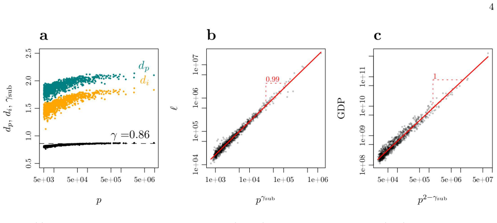
For a city treated as two interlocking fractals, the planar tangle of streets and the three-dimensional cloud of residents, both scaling families follow from eliminating the common linear size $L$ between $\ell\sim L^{d_i}$ and $p\sim L^{d_p}$. The paper's central claim is that the sub-linear exponent is $\gamma_{\rm sub}=d_i/d_p$; that the projected population dimension is empirically close to $d_i$, so interactions within occupied cells give $N\sim p^{2-d_{pp}/d_p}\sim p^{2-\gamma_{\rm sub}}$; and that the equality $\gamma_{\rm sup}=2-\gamma_{\rm sub}$ is therefore a geometric consequence. It further claims the same relation fixes the scaling of average building height, $\langle h\rangle\sim p^{1-\gamma_{\rm sub}}$, and that the data for the largest cities in the UK, with $\gamma_{\rm sub}\simeq0.86$, match road length, GDP, and height scalings to the predicted exponents.

Load-bearing premise

The derivation hinges on estimating the vertical population dimension from average and maximum building heights, and in practice the average height is replaced by a power-law fit to the same volunteered height data that later verifies the height prediction.

Editorial extensions

If this is right

Road network length scales as $p^{\gamma_{\rm sub}}$ with $\gamma_{\rm sub}=d_i/d_p$, so per-capita infrastructure length falls as cities grow.
Total interactions and GDP scale as $p^{2-\gamma_{\rm sub}}$, so per-capita socio-economic output rises with city size, and the two exponents sum to 2.
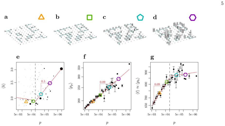
Average building height is predicted to grow as $p^{1-\gamma_{\rm sub}}$ above roughly 100,000 people, with horizontal densification below that threshold.
The scaling exponent is not a single universal constant; it varies with city size, and single-exponent fits depend on the lower population cutoff.
The same ratio reproduces road-length and GDP scaling for France, Germany, Spain, and Italy as well as the UK.

Reading between the lines

Editorial extensions of the paper, not claims the author makes directly.

The paper does not state, but its logic implies, that the city-boundary problem is less severe for the ratio than for either dimension alone: if boundaries shift, $d_i$ and $d_p$ should move together, keeping $\gamma_{\rm sub}$ comparatively stable.
A testable extension is to apply the same ratio to non-European cities using direct measurements of building heights; cities with different vertical building distributions should show different $\gamma_{\rm sub}$ values, and the framework predicts road-length scaling changes accordingly.
The critical population near 100,000 is treated empirically; a natural question is whether it coincides with the transition from monocentric to polycentric cities, which could be checked against commuting-flow data.
If the height prediction is correct, then urban density limits are geometric: once heights saturate, the road network must densify further or the city must develop new centres.

Share X Bluesky LinkedIn Reddit HN

Signed reviews

No signed human review yet.

Editorial analysis

A structured set of objections, weighed in public.

Desk editor's note, referee report, and a circularity audit.

Desk Editor's Note

read the letter

Short version: this is a genuinely elegant geometric derivation of the two urban scaling exponents, and the data work is mostly transparent, but the headline 'prediction' about building heights is partly circular, and the numerical validation is weaker than the text claims. Worth engaging, but it needs a revision that recomputes the population fractal dimension from raw height data and treats the height scaling as a real out-of-sample test.

What's actually new: the sub-linear exponent as γ_sub = d_i/d_p, with d_p including a vertical component, is a clean extension of Bettencourt's framework. The height prediction ⟨h⟩ ∼ p^{1−γ_sub} with a transition around 100,000 people is concrete and falsifiable, and the point that γ_sub varies with city size is a useful explanation for why single-exponent fits are unstable. The dataset is large, and the percolation-based city boundary method is a solid contribution.

The soft spots are real but not fatal. The height prediction is not as independent as it looks. In SI §9b the authors replace measured ⟨h⟩ and h_m with global power-law fits, then use those fits to estimate d_p via Eq. 13, which sets γ_sub. The 'verification' in Fig. 3e then compares the derived 1−γ_sub to the slope from the same fitted curve. That is not an independent confirmation. The reported slope is 0.10 versus a predicted 0.14, which is a visible miss, not a clean hit. The two-point estimate of d_p is crude, and h_m is a maximum statistic, exactly where the acknowledged OSM bias toward tall buildings in big cities would bite. The GDP plot is a consistency check, not an independent fit, and the 100k threshold is chosen from the data. None of this kills the central idea, but it lowers the evidential weight.

My take: the geometric ratio is probably right in spirit, and the paper deserves a serious referee. The fix is straightforward: compute d_p from raw heights per city, report bootstrap uncertainties, and test the height prediction on a holdout set or at least with a fit that does not feed back into d_p. I'd engage with it.

Referee Report

3 major / 5 minor

Summary. The paper proposes that urban sub-linear scaling of infrastructure with population follows from the ratio of two fractal dimensions: the road network dimension d_i and the 3D population dimension d_p, so γ_sub=d_i/d_p. Super-linear scaling is derived from pairwise interactions in 1×1 squares, giving γ_sup=2−γ_sub. The authors further predict that average building height scales as ⟨h⟩∼p^{1−γ_sub} above a critical population, and they test this with OpenStreetMap height data for UK cities, alongside road length, GDP, projected population, and area for 4750 European cities. The main text and SI present a dimensional derivation plus empirical validation based on box-counting of road networks and a two-point estimate of d_p from building heights.

Significance. If the central dimensional relation holds, the framework is valuable because it converts the observed near-universal urban scaling exponents into concrete geometric ratios and yields falsifiable predictions about building heights. The explicit derivations of ℓ∼p^{γ_sub}, N∼p^{2−γ_sub}, and ⟨h⟩∼p^{1−γ_sub} are clear and mostly self-contained, and the multi-country dataset is a strength. The empirical links among road networks, projected population, and GDP give the proposal genuine reach. The significance is conditional, however: the height-based determination of d_p is not yet an independent measurement, so the claimed confirmation of the height prediction is weaker than the paper presents.

major comments (3)

[SI §9b and Eq. (13)] The estimate of d_p is not independent of the height scaling it is used to verify. The authors replace per-city ⟨h⟩ and h_m with global power-law fits ⟨h⟩=⟨h⟩_0 p^α and h_m=h_{m,0}p^η (SI §9b, Fig. 13), then insert these fitted values into SI Eq. (13). Consequently γ_sub=d_i/d_p inherits the fitted exponent α, and the predicted height exponent 1−γ_sub is compared in Fig. 3(e) and Table I with the slope α from the same fitted curve. I ask for a recomputation using raw per-city heights and for reported uncertainties on α, η, and γ_sub.
[Table I and Fig. 3(e)] The reported numbers do not match the theory. With γ_sub=0.86 the prediction is 1−γ_sub=0.14, while Fig. 3(e) reports a measured slope of 0.10 and Fig. 3(f) reports 0.09; Table I lists the measured height exponent as 0.10. The manuscript does not discuss this 0.04 gap or provide confidence intervals. Please give the statistical uncertainty on both the predicted and measured exponents and explain whether the difference is consistent with the acknowledged OSM height bias and with the choice of the 100,000-person threshold.
[SI §4b] The two-box estimate in Eq. (13), d_p = d_pp + log⟨h⟩/log h_m, uses h_m, a maximum statistic that is especially sensitive to the OSM sampling bias toward important buildings in large cities that the authors themselves acknowledge in SI §9b. Since every derived exponent (γ_sub, γ_sup, and the height exponent) flows through d_p, the paper needs a sensitivity check, for example using a high quantile instead of the maximum, or restricting to cities with fuller OSM coverage, before the exponent predictions can be considered robust.

minor comments (5)

[Table I] The column arrangement is hard to read; '1 − γ_sub' and '0.10' are not clearly separated into theory and measured columns. Please reformat the table so each column is unambiguous.
[SI Fig. 10 caption] The caption says 'Same setting as in Fig. 3 in the main text' for the UK dimensions, but the UK dimensions are shown in main-text Fig. 2; please correct the cross-reference.
[Title] The title contains a typo ('de termines'); please fix it.
[Main text, after Eq. (5)] The interaction count assumes the square of the number of people per unit square; this is an explicit modeling assumption rather than a consequence of the geometry, and it should be flagged as such in the derivation.
[SI §9b] The statement that improved height data 'might slightly alter the results' should be quantified, since the height fits are load-bearing for d_p.

Circularity Check

1 steps flagged · score 6.0 of 10

Height scaling 'prediction' is partly circular: d_p is built from power-law fits to the same ⟨h⟩ data later used to 'verify' ⟨h⟩ ~ p^{1−γ_sub}; the central geometric ratio is otherwise independent.

fitted input called prediction [SI §4b, Eq. 13; SI §9b; main text Eq. 6 and Fig. 3(e)]
"dp ∼ log⟨p⟩3hm − log⟨p⟩3 / log 3hm − log 3 = dpp + log⟨h⟩/log hm ... Given the low quality of the data relating to the heights of buildings, we substituted the average number of levels, ⟨h⟩, of each city and the maximum heights, hm, with power-laws with respect to p by fitting the two variables. ... you obtain the final approximation according to ⟨h⟩ = ⟨h⟩0p^α. The same is done for hm. ... follows the theoretical prediction for the exponent 1 − γsub."

The 3D population dimension d_p is not measured directly: SI Eq. 13 defines it as d_pp + log⟨h⟩/log h_m. SI §9b then substitutes both per-city height inputs by global power-law fits ⟨h⟩=⟨h⟩0 p^α and h_m=h_{m,0} p^η. Since γ_sub = d_i/d_p, the predicted height exponent 1−γ_sub is a function of the fitted height slope α (with d_pp≈d_i, 1−γ_sub≈α/(ηd_i+α)). The 'prediction' ⟨h⟩∼p^{1−γ_sub} in Eq. 6 therefore inherits a parameter fitted to the same ⟨h⟩ data that Fig. 3(e) uses for confirmation (slope 0.10). This is not an independent test; it is a consistency check on the height fit, and the acknowledged OSM height bias makes the fitted input load-bearing.

full rationale

The central geometric claim γ_sub = d_i/d_p is not itself circular: d_i is box-counted from street networks and d_pp from population grids, and the derivation ℓ ∼ p^{d_i/d_p} is a nontrivial algebraic consequence that could in principle be rejected by data. The super-linear relation and the addition law γ_sup = 2−γ_sub are also derived, not fitted. The circularity is localized to the height prediction. Because d_p is estimated from average and maximum building heights (SI Eq. 13), and because SI §9b replaces those heights with power-law fits in p before computing d_p, the predicted height exponent 1−γ_sub depends on the fitted height slope α. Confirming that same height data grows as p^{1−γ_sub} is therefore a consistency check rather than an independent validation. The paper's self-citation [48] concerns city-boundary methodology and is not load-bearing for the exponent claims. The acknowledged OSM height bias and the two-point nature of the height contribution to d_p further weaken this particular prediction, but do not make the whole derivation circular. Overall: partial circularity affecting one highlighted prediction, score 6.

Assumptions & free parameters 5 free parameters · 6 assumptions · 0 invented entities

The framework rests on a few geometric scaling ansatze (monofractality, d_pp = d_i) and two strong behavioral assumptions (pairwise interactions in unit cells; constant people per floor per road length). The 3D population fractal dimension is not directly measured but inferred from height power-law fits, so the apparent predictive power is partly inherited from those fits.

free parameters (5)

height power-law prefactor ⟨h⟩0 = not reported (fit in SI Fig. 13)
The average number of building levels in each city is replaced by the fitted function ⟨h⟩ = ⟨h⟩0 p^α (SI 9b). This fitted prefactor enters the estimate of d_p through SI Eq. 13, hence affects γ_sub and the predicted exponents.
height power-law exponent α = ~0.10 (reported slope, Fig. 3e)
The exponent α is estimated by weighted regression on cities above 100,000 people and is used, via ⟨h⟩ in SI Eq. 13, to compute d_p. The same α is then presented as the empirical confirmation of the predicted height scaling 1−γ_sub.
maximum height power-law prefactor h_{m,0} = not reported
The maximum building height h_m per city is replaced by a power-law fit h_m = h_{m,0} p^α_m (SI 9b), which enters the denominator of β = log⟨h⟩/log h_m in SI Eq. 13.
maximum height power-law exponent α_m = not reported
This exponent controls the p-dependence of h_m in the estimate of the vertical fractal component β; it therefore shapes γ_sub(p) and the size-dependence claim.
critical population threshold = about 100,000 people
The threshold above which height scaling is observed and the regime-change claim is made is chosen from the data (Fig. 3e-g), not derived from the geometry.

assumptions (6)

domain assumption The street network and the population distribution are monofractals with well-defined single box-counting dimensions d_i and d_p over the range 150 to 500 m.
Used throughout; the box-counting limits are imposed in SI section 3 because the data curve below 150 m and saturate above 500 m.
domain assumption The fractal dimension of the projected population equals that of the street network, d_pp = d_i.
Assumed in the super-linear derivation and height derivation; supported by SI Fig. 8 (regression d_pp = 1.01d_i − 0.10), but treated as an identity in the equations.
ad hoc to paper In a unit square, the number of pairwise interactions is proportional to the square of the number of people in that square.
This is the load-bearing behavioral assumption in the derivation of N ∼ p^{2−γ_sub} (main text Eq. 5); no micro-foundation is given.
ad hoc to paper Average building height is proportional to total population divided by total road length, with constant people per floor and building depth.
Used to derive ⟨h⟩ ∼ p/ℓ ∼ p^{1−γ_sub} (main text around Eq. 6); the constancy of people per floor and building depth is stated as an assumption but not tested.
domain assumption City boundaries are defined by the percolation threshold that maximizes the population-weighted average fractal dimension of clusters.
This methodological choice (SI section 2) sets which spatial units are called cities; because the threshold is chosen by maximizing a fractal dimension, it can bias the very dimensions used later.
ad hoc to paper The vertical component of the population fractal, β, can be estimated as log⟨h⟩/log h_m.
Introduced in SI section 4b with only two box sizes (floor height 3 m and maximum height 3 h_m); this is a minimal two-point box-counting estimate, not a measured scaling law.

how reviews work

0 comments

Cite this review

Pith. "Pith review of How the geometry of cities explains urban scaling laws and determines their exponents." pith.science (2026). https://pith.science/paper/OX3THBKH

@misc{pith2026190807470,
  author       = {Pith},
  title        = {Pith review of: How the geometry of cities explains urban scaling laws and determines their exponents},
  year         = {2026},
  howpublished = {\url{https://pith.science/paper/OX3THBKH}},
  note         = {Machine review of arXiv:1908.07470}
}

read the original abstract

Urban scaling laws relate socio-economic, behavioral, and physical variables to the population size of cities and allow for a new paradigm of city planning, and an understanding of urban resilience and economies. Independently of culture and climate, almost all cities exhibit two fundamental scaling exponents, one sub-linear and one super-linear that are related. Here we show that based on fundamental fractal geometric relations of cities we derive both exponents and their relation. Sub-linear scaling arises as the ratio of the fractal dimensions of the road network and the distribution of the population in 3D. Super-linear scaling emerges from human interactions that are constrained by the city geometry. We demonstrate the validity of the framework with data on 4750 European cities. We make several testable predictions, including the relation of average height of cities with population size, and that at a critical population size, growth changes from horizontal densification to three-dimensional growth.

Figures

Figures reproduced from arXiv: 1908.07470 by the authors.

**Figure 2.** (a) Fractal dimensions of the street network, [PITH_FULL_IMAGE:figures/full_fig_p004_2.png] view at source ↗

**Figure 3.** Schematic illustration of how a city grows. (a)-(b [PITH_FULL_IMAGE:figures/full_fig_p005_3.png] view at source ↗

Figures from the paper (11 more)

**Figure 4.** Figure 4: Showing the implications of the dependence of [PITH_FULL_IMAGE:figures/full_fig_p008_4.png]

**Figure 5.** Figure 5: Showing how the curvature of ℓ is corrected through the calculated γsub. (a) linear regression between ℓ and γsub for the whole set of cities. (b) Slopes of the linear regressions between ℓ and γsub for increasingly larger sets of cities, showing how the relationship i…

**Figure 6.** Figure 6: Methodology to construct the network of the popula [PITH_FULL_IMAGE:figures/full_fig_p010_6.png]

**Figure 7.** Figure 7: Determining the threshold to obtain cities. (a) we [PITH_FULL_IMAGE:figures/full_fig_p011_7.png]

**Figure 8.** Figure 8: Fractal dimension of the population, dpp , versus the dimension of the street network, di. It is seen that the two dimensions practically align. The red line represents the linear regression. 5. Derivation of the relation between ℓ and p with proportionality factors Gi…

**Figure 9.** Figure 9: (a) Approximation of the area with N 2/di l,250. (b) The relation between ℓ and its approximated version using the length of the city L di . (c) Similar approximation between p and L dp . Green lines denote a perfect relation with a slope of 1. 7. Results for FR, DE, E…

**Figure 10.** Figure 10: Fractal dimensions of the street network, [PITH_FULL_IMAGE:figures/full_fig_p016_10.png]

**Figure 11.** Figure 11: Correspondance between hhi and hppi and p 1−γsub . (a) p 1−γsub in black (grey are the true values, black points represent its local averages), and hhi where the size and thickness represent the number of buildings. (b) p 1−γsub in black (grey are the true values, bla…

**Figure 12.** Figure 12: The data sources used in this work include, (a) pop [PITH_FULL_IMAGE:figures/full_fig_p017_12.png]

**Figure 13.** Figure 13: Substituting the number of levels by power-laws, [PITH_FULL_IMAGE:figures/full_fig_p018_13.png]

**Figure 14.** Figure 14: Relationship between the area and the population [PITH_FULL_IMAGE:figures/full_fig_p018_14.png]

Discussion (0). Continue with ORCID to comment.

Reference graph

Works this paper leans on

67 extracted references · 65 canonical work pages

[1]

With Eqs

The total number of interactions N in a city in a single in- stant would be that value, multiplied by the number of locations in which that can happen, which is Ldpp . With Eqs. (

work page
[2]

(4) We can now estimate the number of interactions

and ( 3), we can now write ⟨pp⟩1 = ⟨p⟩1Ldp−dpp . (4) We can now estimate the number of interactions. If we have ⟨pp⟩1 people in a square of size 1, the maximal num- ber of their interactions is ⟨pp⟩1(⟨pp⟩1 − 1) ∼ ⟨pp⟩2

work page
[3]

Barthelemy, The Structure and Dynamics of Cities: Urban Data Analysis and Theoretical Modeling

M. Barthelemy, The Structure and Dynamics of Cities: Urban Data Analysis and Theoretical Modeling . Cam- bridge University Press, 2016

work page 2016
[4]

(5) Here we used our empirical ﬁnding that the fractal dimen- sion of the projected population follows the dimension of the street network, dpp ∼ di; see SI Fig

and ( 2) we get N ∼ ⟨pp⟩2 1Ldpp ∼ L2dp−dpp ∼ p2− dpp dp ∼ p2−γsub . (5) Here we used our empirical ﬁnding that the fractal dimen- sion of the projected population follows the dimension of the street network, dpp ∼ di; see SI Fig

work page
[5]

Batty, The new science of cities

M. Batty, The new science of cities . Mit Press, 2013

work page 2013
[6]

G. B. West, Scale: the universal laws of growth, inno- vation, sustainability, and the pace of life in organisms, cities, economies, and companies . Penguin, 2017

work page 2017
[7]

Scaling laws in urban supply networks,

C. Kühnert, D. Helbing, and G. B. West, “Scaling laws in urban supply networks,” Physica A: Statistical Mechanics and its Applications , vol. 363, no. 1, pp. 96–103, 2006

work page 2006
[8]

The addi- tion rule follows from this derivation

We identify the scaling exponent obtained from interaction densities as the super-linear exponent, γsup = 2 − γsub. The addi- tion rule follows from this derivation. As an example for a known super-linear quantity, we show the actual GDP for UK cites in comparison to the theoretical prediction in Fig. 2 c. City GDP data was obtained from [ 43] and is desc...

work page

Show all 67 references

[9]

Scaling laws in urban sys- tems,

D. Pumain and M. Guerois, “Scaling laws in urban sys- tems,” in Santa Fe Institute, Working Papers , p. 4, 2004

2004
[10]

The scaling of green space coverage in european cities,

R. A. Fuller and K. J. Gaston, “The scaling of green space coverage in european cities,” Biology letters, vol. 5, no. 3, pp. 352–355, 2009

2009
[11]

Urban scaling and its deviations: Revealing the structure of wealth, innovation and crime across cities,

L. M. Bettencourt, J. Lobo, D. Strumsky, and G. B. West, “Urban scaling and its deviations: Revealing the structure of wealth, innovation and crime across cities,” PloS one , vol. 5, no. 11, p. e13541, 2010

2010
[12]

Optimal design of spa- tial distribution networks,

M. T. Gastner and M. Newman, “Optimal design of spa- tial distribution networks,” Physical Review E , vol. 74, no. 1, p. 016117, 2006

2006
[13]

Growth, innovation, scaling, and the pace of life in cities,

L. M. Bettencourt, J. Lobo, D. Helbing, C. Kühnert, and G. B. West, “Growth, innovation, scaling, and the pace of life in cities,” Proceedings of the national academy of sciences, vol. 104, no. 17, pp. 7301–7306, 2007

2007
[14]

Rich and poor cities in europe. an urban scaling approach to mapping the european eco- nomic transition,

E. Strano and V. Sood, “Rich and poor cities in europe. an urban scaling approach to mapping the european eco- nomic transition,” PloS one , vol. 11, no. 8, p. e0159465, 2016

2016
[15]

Invention in the city: Increasing returns to patenting as a scaling function of metropolitan size,

L. M. Bettencourt, J. Lobo, and D. Strumsky, “Invention in the city: Increasing returns to patenting as a scaling function of metropolitan size,” Research policy, vol. 36, no. 1, pp. 107–120, 2007

2007
[16]

A tale of many cities: universal patterns in human urban mobility,

A. Noulas, S. Scellato, R. Lambiotte, M. Pontil, and C. Mascolo, “A tale of many cities: universal patterns in human urban mobility,” PloS one, vol. 7, no. 5, p. e37027, 2012

2012
[17]

Cities as organisms: Allometric scaling of urban road networks,

H. Samaniego and M. E. Moses, “Cities as organisms: Allometric scaling of urban road networks,” Journal of Transport and Land use , vol. 1, no. 1, pp. 21–39, 2008

2008
[18]

Is this scaling nonlinear?,

J. C. Leitão, J. M. Miotto, M. Gerlach, and E. G. Alt- mann, “Is this scaling nonlinear?,” Royal Society open science, vol. 3, no. 7, p. 150649, 2016

2016
[19]

Scaling and hierarchy in urban economies,

C. R. Shalizi, “Scaling and hierarchy in urban economies,” arXiv preprint arXiv:1102.4101 , 2011

2011 arXiv
[20]

Constructing cities, deconstructing scaling laws,

E. Arcaute, E. Hatna, P. Ferguson, H. Youn, A. Johans- son, and M. Batty, “Constructing cities, deconstructing scaling laws,” Journal of The Royal Society Interface , vol. 12, no. 102, p. 20140745, 2015

2015
[21]

Di- verse cities or the systematic paradox of urban scal- ing laws,

C. Cottineau, E. Hatna, E. Arcaute, and M. Batty, “Di- verse cities or the systematic paradox of urban scal- ing laws,” Computers, Environment and Urban Systems , 7 vol. 63, pp. 80–94, 2017

2017
[22]

Scaling: lost in the smog,

R. Louf and M. Barthelemy, “Scaling: lost in the smog,” Environment and Planning B: Planning and Design , vol. 41, no. 5, pp. 767–769, 2014

2014
[23]

A uniﬁed theory of urban living,

L. Bettencourt and G. West, “A uniﬁed theory of urban living,” Nature, vol. 467, no. 7318, p. 912, 2010

2010
[24]

A model of urban scaling laws based on distance de- pendent interactions,

F. L. Ribeiro, J. Meirelles, F. F. Ferreira, and C. R. Neto, “A model of urban scaling laws based on distance de- pendent interactions,” Royal Society open science , vol. 4, no. 3, p. 160926, 2017

2017
[25]

Thurner, R

S. Thurner, R. Hanel, and P. Klimek, Introduction to the Theory of Complex Systems . Oxford University Press, 2018

2018
[26]

The origins of scaling in cities,

L. M. Bettencourt, “The origins of scaling in cities,” sci- ence, vol. 340, no. 6139, pp. 1438–1441, 2013

2013
[27]

Su- perlinear scaling for innovation in cities,

S. Arbesman, J. M. Kleinberg, and S. H. Strogatz, “Su- perlinear scaling for innovation in cities,” Physical Review E, vol. 79, no. 1, p. 016115, 2009

2009
[28]

Superlinear and sublinear urban scaling in geographical networks model- ing cities,

K. Yakubo, Y. Saijo, and D. Korošak, “Superlinear and sublinear urban scaling in geographical networks model- ing cities,” Physical Review E , vol. 90, no. 2, p. 022803, 2014

2014
[29]

An evolutionary theory for interpreting urban scaling laws,

D. Pumain, F. Paulus, C. Vacchiani-Marcuzzo, and J. Lobo, “An evolutionary theory for interpreting urban scaling laws,” Cybergeo: European Journal of Geography , 2006

2006
[30]

Multifractal to monofractal evolution of the london street network,

R. Murcio, A. P. Masucci, E. Arcaute, and M. Batty, “Multifractal to monofractal evolution of the london street network,” Physical Review E , vol. 92, no. 6, p. 062130, 2015

2015
[31]

Batty and P

M. Batty and P. A. Longley, Fractal cities: a geometry of form and function . Academic press, 1994

1994
[32]

Fractal properties of settlement struc- tures,

P. Frankhauser, “Fractal properties of settlement struc- tures,” in First International Seminar on Structural Mor- phology, 1992

1992
[33]

Aspects fractals des structures ur- baines,

P. Frankhauser, “Aspects fractals des structures ur- baines,” L’Espace géographique, pp. 45–69, 1990

1990
[34]

Urban shapes as fractals,

M. Batty and P. A. Longley, “Urban shapes as fractals,” Area, pp. 215–221, 1987

1987
[35]

Fractal-based description of urban form,

M. Batty and P. A. Longley, “Fractal-based description of urban form,” Environment and planning B: Planning and Design , vol. 14, no. 2, pp. 123–134, 1987

1987
[36]

Scaling in biology: the con- sequences of size,

K. Schmidt-Nielsen, “Scaling in biology: the con- sequences of size,” Journal of Experimental Zoology , vol. 194, no. 1, pp. 287–307, 1975

1975
[37]

A general model for the origin of allometric scaling laws in biology,

G. B. West, J. H. Brown, and B. J. Enquist, “A general model for the origin of allometric scaling laws in biology,” Science, vol. 276, no. 5309, pp. 122–126, 1997

1997
[38]

The fourth dimension of life: fractal geometry and allometric scaling of organisms,

G. B. West, J. H. Brown, and B. J. Enquist, “The fourth dimension of life: fractal geometry and allometric scaling of organisms,” science, vol. 284, no. 5420, pp. 1677–1679, 1999

1999
[39]

A general model for ontogenetic growth,

G. B. West, J. H. Brown, and B. J. Enquist, “A general model for ontogenetic growth,” Nature, vol. 413, no. 6856, p. 628, 2001

2001
[40]

Ur- ban growth and form: scaling, fractal geometry, and diﬀusion-limited aggregation,

M. Batty, P. Longley, and S. Fotheringham, “Ur- ban growth and form: scaling, fractal geometry, and diﬀusion-limited aggregation,” Environment and Plan- ning A , vol. 21, no. 11, pp. 1447–1472, 1989

1989
[41]

Batty and P

M. Batty and P. Longley, Fractal Cities: A Geometry of Form and Function. Academic Press, San Diego, CA and London, 1994

1994
[42]

The size, scale, and shape of cities,

M. Batty, “The size, scale, and shape of cities,” science, vol. 319, no. 5864, pp. 769–771, 2008

2008
[43]

The fractal approach. a new tool for the spatial analysis of urban agglomerations,

P. Frankhauser, “The fractal approach. a new tool for the spatial analysis of urban agglomerations,” Population: an english selection , pp. 205–240, 1998

1998
[44]

Global human settlement layer. pop- ulation grid, european commission

“Global human settlement layer. pop- ulation grid, european commission.” http://ghsl.jrc.ec.europa.eu/ghs_pop.php, 2015

2015
[45]

Planet dump retrieved from https://planet.osm.org

OpenStreetMap contributors, “Planet dump retrieved from https://planet.osm.org .” https://www.openstreetmap.org, 2017

2017
[46]

The scaling of human interactions with city size,

M. Schläpfer, L. M. Bettencourt, S. Grauwin, M. Raschke, R. Claxton, Z. Smoreda, G. B. West, and C. Ratti, “The scaling of human interactions with city size,” Journal of the Royal Society Interface , vol. 11, no. 98, p. 20130789, 2014

2014
[47]

Eurostat gdp data at nuts-3 level

“Eurostat gdp data at nuts-3 level.” https://ec.europa.eu/eurostat/web/rural-development/data
[48]

Urban sky- lines: building heights and shapes as measures of city size,

M. Schläpfer, J. Lee, and L. Bettencourt, “Urban sky- lines: building heights and shapes as measures of city size,” arXiv preprint arXiv:1512.00946 , 2015

2015 arXiv
[49]

Modeling the polycentric transition of cities,

R. Louf and M. Barthelemy, “Modeling the polycentric transition of cities,” Physical review letters , vol. 111, no. 19, p. 198702, 2013

2013
[50]

How congestion shapes cities: from mobility patterns to scaling,

R. Louf and M. Barthelemy, “How congestion shapes cities: from mobility patterns to scaling,” Scientiﬁc re- ports, vol. 4, p. 5561, 2014

2014
[51]

Urban scaling in eu- rope,

L. M. Bettencourt and J. Lobo, “Urban scaling in eu- rope,” Journal of The Royal Society Interface , vol. 13, no. 116, p. 20160005, 2016

2016
[52]

Cities and regions in britain through hierarchical percolation,

E. Arcaute, C. Molinero, E. Hatna, R. Murcio, C. Vargas- Ruiz, A. P. Masucci, and M. Batty, “Cities and regions in britain through hierarchical percolation,” Royal Society Open Science, vol. 3, no. 4, 2016

2016
[53]

Stauﬀer and A

D. Stauﬀer and A. Aharony, Introduction to Percolation Theory. London: Taylor and Francis, 1994

1994
[54]

Laws of population growth,

H. D. Rozenfeld, D. Rybski, J. S. Andrade, M. Batty, H. E. Stanley, and H. A. Makse, “Laws of population growth,” Proceedings of the National Academy of Sci- ences, vol. 105, no. 48, pp. 18702–18707, 2008

2008
[55]

The area and population of cities: New insights from a diﬀerent perspective on cities,

H. D. Rozenfeld, D. Rybski, X. Gabaix, and H. A. Makse, “The area and population of cities: New insights from a diﬀerent perspective on cities,” American Economic Re- view, vol. 101, no. 5, pp. 2205–25, 2011

2011
[56]

Falconer, Fractal geometry: mathematical foundations and applications

K. Falconer, Fractal geometry: mathematical foundations and applications. John Wiley & Sons, 2004

2004
[57]

Percolation theory,

K. Christensen, “Percolation theory,” Imperial College London, vol. 1, 2002. 8 Figure 4. Showing the implications of the dependence of γsub on the population. (a) Represents a linear regression (in a l og-log scale) for all cities in the UK. (b) Shows the values of the exp one...

2002
[58]

After all, the variation is numerically very small and even we have done the same in this work for summarisi ng purposes

Describing the dependence of the scaling exponent on the p opulation In order to depict and calculate the exponent of the scaling, it is common to use a single number for each system of cities as if the behaviour among cities of diﬀerent sizes wou ld be constant. After all, th...
[59]

The approach allows us to meaningfully compare cities with each other, and also a cross countries

Deﬁnition of city boundaries We base the deﬁnition of cities on a set of systematic criteri a obtained from population data. The approach allows us to meaningfully compare cities with each other, and also a cross countries. Previous work [ 48] laid out the basic building block...
[60]

Measuring fractal dimensions: box-counting for the stre et network After obtaining the area that each city occupies we extract i ts roads from the planet ﬁle of Open Street Maps [ 41] and calculate the box-counting dimension [ 52]. A standard algorithm for calculating this dim...
[61]

Estimating the fractal dimension of the population The basic idea is to decompose dp = dpp + β into a planar (or projected) part, dpp , and a component that captures the fractality β of the height of buildings, which can be approximated from da ta on the number of levels of th...
[62]

Derivation of the relation between ℓ and p with proportionality factors Given squares of length ǫ, the average length of the street network inside each square can be written as ⟨ℓ⟩ǫ = kiǫdi . (15) In the same spirit, we can view the population distributed in space as a cloud o...
[63]

Validity of the approximations We show in Fig. 9 (b) how the approximated values to ℓ and p as a function of the city length scale behave, showing that even though it remains an approximation the values are q uite close to the real measurement. L is the theoretical linear leng...
[64]

Results for FR, DE, ES, IT We show in Fig. 10 the fractal dimensions for the street network, di, and the population, dp, as measured with box- counting and the estimation described above for France (FR) , Germany (DE), Spain (ES), and Italy (IT). Germany presents such bad aver...
[65]

11 how the the average number of levels in cities ⟨h⟩, its projected population ⟨pp⟩ both follow the same behaviour which is characterised by p1−γsub

Correspondance between ⟨h⟩ and ⟨pp⟩ We show in Fig. 11 how the the average number of levels in cities ⟨h⟩, its projected population ⟨pp⟩ both follow the same behaviour which is characterised by p1−γsub
[66]

important

Datasets a. Population data We use the Global Human Settlement (GHS) Population Grid fro m 2015 [40], which is a global map of the population with a resolution of 250 × 250m, produced by the European Commission, see Fig. 12 (a). From this dataset we obtain the city boundaries ...

2015
[67]

14 we show the measurement of the relationship between the area and the population

Relation between area and population In Fig. 14 we show the measurement of the relationship between the area and the population. 16 France Germany Spain Italy Figure 10. Fractal dimensions of the street network, di, (orange) and for the population, dp (blue), for cities in Fra...

Pith tools

Reviewed August 14, 2026 · model on record in the stance chip above.

[1] [1]

With Eqs

The total number of interactions N in a city in a single in- stant would be that value, multiplied by the number of locations in which that can happen, which is Ldpp . With Eqs. (

work page

[2] [2]

(4) We can now estimate the number of interactions

and ( 3), we can now write ⟨pp⟩1 = ⟨p⟩1Ldp−dpp . (4) We can now estimate the number of interactions. If we have ⟨pp⟩1 people in a square of size 1, the maximal num- ber of their interactions is ⟨pp⟩1(⟨pp⟩1 − 1) ∼ ⟨pp⟩2

work page

[3] [3]

Barthelemy, The Structure and Dynamics of Cities: Urban Data Analysis and Theoretical Modeling

M. Barthelemy, The Structure and Dynamics of Cities: Urban Data Analysis and Theoretical Modeling . Cam- bridge University Press, 2016

work page 2016

[4] [4]

(5) Here we used our empirical ﬁnding that the fractal dimen- sion of the projected population follows the dimension of the street network, dpp ∼ di; see SI Fig

and ( 2) we get N ∼ ⟨pp⟩2 1Ldpp ∼ L2dp−dpp ∼ p2− dpp dp ∼ p2−γsub . (5) Here we used our empirical ﬁnding that the fractal dimen- sion of the projected population follows the dimension of the street network, dpp ∼ di; see SI Fig

work page

[5] [5]

Batty, The new science of cities

M. Batty, The new science of cities . Mit Press, 2013

work page 2013

[6] [6]

G. B. West, Scale: the universal laws of growth, inno- vation, sustainability, and the pace of life in organisms, cities, economies, and companies . Penguin, 2017

work page 2017

[7] [7]

Scaling laws in urban supply networks,

C. Kühnert, D. Helbing, and G. B. West, “Scaling laws in urban supply networks,” Physica A: Statistical Mechanics and its Applications , vol. 363, no. 1, pp. 96–103, 2006

work page 2006

[8] [8]

The addi- tion rule follows from this derivation

We identify the scaling exponent obtained from interaction densities as the super-linear exponent, γsup = 2 − γsub. The addi- tion rule follows from this derivation. As an example for a known super-linear quantity, we show the actual GDP for UK cites in comparison to the theoretical prediction in Fig. 2 c. City GDP data was obtained from [ 43] and is desc...

work page