Stochastic regularity of general quadratic observables of high frequency waves

Gabriela Malenova; Olof Runborg

Stochastic regularity of general quadratic observables of high frequency waves

T0 review · 0 major / 5 minor · reviewed 2026-08-14 · deepseek-v4-flash

Challenge this review Re-run · record.json Download PDF Read on arXiv ↗ Review JSON

Pith's one-line read The paper proves that time-averaged quadratic observables of high-frequency waves, computed by Gaussian beams, have parameter derivatives uniformly bounded as the wavelength tends to zero.

desk verdict Solid, honest generalization of the authors' earlier one-mode regularity result to the two-mode time-averaged case; the core estimates check out and it deserves a serious referee with minor revisions. read the letter →

arxiv 1908.07472 v1 pith:3NERD5QC submitted 2019-08-20 math.NA cs.NA

Gabriela Malenova , Olof Runborg This is my paper · ORCID

classification math.NAcs.NA MSC 65M9935L0560H35

keywords stochasticregularityGaussianbeamshigh-frequencywavesuncertaintyquantificationquadraticobservablessparsegridcollocationwaveequationnon-stationaryphase

verification ladder T0 review T1 audit T2 compute T3 formal

The pith

A machine-rendered reading of the paper's core claim, the machinery that carries it, and where it could break.

The reading

High-frequency wave fields oscillate on a scale $\varepsilon$, and quantities computed from them typically inherit that oscillation, making their dependence on uncertain parameters increasingly rough as $\varepsilon$ shrinks, which is the opposite of what fast stochastic methods require. The paper identifies a class of quadratic observables that escape this problem: weighted space-time integrals of $|\partial_t^p\partial_x^\alpha u|^2$, evaluated on a Gaussian-beam approximation of the wave field. For these observables, every derivative with respect to the stochastic parameters is bounded by a constant independent of $\varepsilon$ (Theorem 5.2), and the same holds for spatial-only one-mode observables uniformly in time (Theorem 4.2). The reason is that the interference term between the two counter-propagating beam modes is killed by time integration through non-stationary phase, so the parameter-to-observable map stays uniformly smooth in the high-frequency limit.

What carries the argument

The argument is carried by the $k$-th order Gaussian beam superposition $u_k=u_k^++u_k^-$, whose phase and amplitude coefficients are solutions of a set of $\varepsilon$-independent ODEs. When the observable is expanded, the difficulty is concentrated in the cross term whose integrand contains the phase $\vartheta_k(t,x,y,z,z')=\Phi_k^-(t,x-q^-,y,z')-(\Phi_k^+)^*(t,x-q^+,y,z)$. Proposition 5.5 shows $|\partial_t\vartheta_k|\ge\nu>0$ on the set where both beams overlap the test function, because the conserved ray Hamiltonians $c(q^\pm)|p^\pm|$ are bounded below by $\gamma>0$ and the beam cutoff width $\mu$ is chosen small enough. The non-stationary phase lemma then bounds the time integral by $\varepsilon^K$ times constants involving derivatives of the amplitude, and the positivity of $\operatorname{Im}\vartheta_k$ from the admissible-cutoff condition gives exponential decay $e^{-\delta|x-q^\pm|^2/\varepsilon}$ outside the overlap. This combination converts every oscillatory integral into an $\varepsilon$-independent bound after taking finitely many derivatives in $y$.

What would settle it

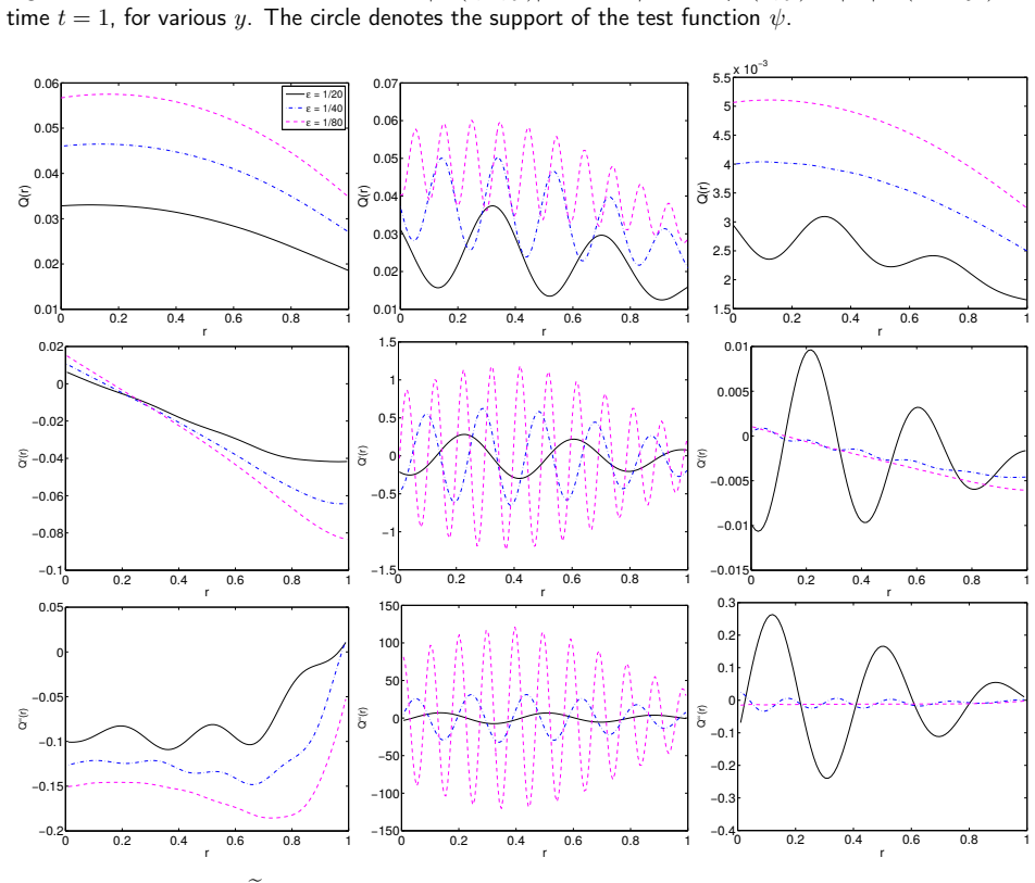
Take the two-mode example in Section 5.4 with $\phi_0=x_1+(x_2-y_1)^2$ and compute $\partial_y^2 Q^{\mathrm{GB}}_{0,0}$ for $\varepsilon = 1/80$, $1/160$, and $1/320$ at the same parameters. Theorem 5.2 predicts the plotted values remain $O(1)$ as $\varepsilon$ shrinks; if the peak values grow like $\varepsilon^{-2}$, the $\varepsilon$-uniformity claim is false.

Watch

Extended reading notes

Core claim

The central result is the $\varepsilon$-uniform stochastic regularity of a general class of quadratic observables. Under assumptions (A1)--(A5), for a fixed final time $T$, beam order $k$, compact parameter set $\Gamma_c$, and an admissible cutoff width $\eta$, the Gaussian-beam observable $$$Q^{{\mathrm{GB}}$}_{p,\$\alpha$}(y)=\$varepsilon^{{2(p+|\alpha|)}}$\int\!\int g(t,x,y)|\partial_t^p\partial_x^\$\alpha$ u_k(t,x,y)|^2\psi(t,x)\,dx\,dt$$ satisfies $\sup_{y\in\Gamma_c}|\partial_y^\sigma Q^{\mathrm{GB}}_{p,\alpha}(y)|\le C_\sigma$, where $C_\sigma$ is independent of $\varepsilon$, for every $p$, multi-index $\alpha$, and derivative multi-index $\sigma$. The one-mode version, with $u_k$ replaced by a single beam family, satisfies the stronger statement that the same bound holds for each fixed time $t\in[0,T]$. The new work beyond the earlier one-mode result is the treatment of the two-mode cross term: the relative phase of the two beams has a time derivative uniformly bounded away from zero wherever both beams reach the measurement window, so the non-stationary phase lemma makes the cross contribution of order $\varepsilon^K$ for any $K$, while Gaussian decay and the cutoffs control everything else.

Load-bearing premise

The two-mode estimate rests on the claim that, whenever both beams reach the measurement region, the relative phase between them changes at a rate that stays strictly positive; this requires the wave speed and the initial phase gradient to be bounded below by positive constants and the beam width to be chosen small enough.

Editorial extensions

If this is right

Sparse-grid stochastic collocation for these observables keeps its fast convergence as $\varepsilon\to0$, because the polynomial and spline interpolation errors in $y$ are controlled by the same $\varepsilon$-independent derivative bounds.
Physical outputs of the form (3), including acoustic potential energy, total energy, and Arias intensity, are covered, so the result applies to seismic and acoustical quantities of interest used in practice.
When one mode dominates, the spatial-only observable is regular at every fixed time, allowing time-dependent statistics without temporal averaging.
The estimates hold for arbitrarily high derivatives in the stochastic parameters, so refinement algorithms that estimate error from higher derivatives will not see $\varepsilon$-dependent growth for these outputs.

Reading between the lines

Editorial extensions of the paper, not claims the author makes directly.

Editor's extension: the same cross-term mechanism should cover bilinear observables such as $\varepsilon^{2m}\int\!\int g\,\overline{D^m u}\,D^m v$ for two different solutions, since only the smooth amplitude changes and the phase difference has the same structure.
Editor's extension: the uniform positivity of $\partial_t\vartheta_k$ is a no-resonance condition; in media with periodic structure or with beams that turn around, stationary phase points can appear, and one would expect $\varepsilon$-dependent observables unless additional averaging in space or parameters is introduced.
Editor's extension: because the proof only uses the sign and size of the conserved ray Hamiltonians, the result should extend to systems of hyperbolic equations and to Schrödinger-type equations whose characteristics have conserved group speeds; the analogous phase derivative would be a difference of group velocities.

Share X Bluesky LinkedIn Reddit HN

Signed reviews

No signed human review yet.

Editorial analysis

A structured set of objections, weighed in public.

Desk editor's note, referee report, and a circularity audit.

Desk Editor's Note

read the letter

Dear colleague,

Read it. The genuinely new content is in Section 5: for a two-mode Gaussian beam superposition, the quadratic observable becomes non-oscillatory when averaged in time, because the cross-term phase has no stationary point in t. The paper proves epsilon-uniform bounds on all parameter derivatives for arbitrary derivative orders p, alpha, and it handles both the one-mode case (extending the earlier p=alpha=0 result) and the two-mode case. The main mechanism is clean: scaled beam derivative classes plus non-stationary phase with tracked constants. I checked the places where a proof like this usually fails, and the argument holds up.

What the paper does well: it identifies a real obstacle (oscillatory cross terms for opposite-propagating modes), gives a simple 1D example showing the failure, and then shows the time-averaging cure is not just heuristic but provable under assumptions (A1)-(A5). The numerical experiments are consistent with the theorems. The self-citations to [22,23,24] are substantial but legitimate: those results are published with proofs, and the new theorems do not assume their own conclusion.

Soft spots, in proportion. The biggest one for a standalone reader is delegation: Theorem 4.6, the one-mode workhorse, is proved by saying "same as Theorem 1 in [23]" plus an appendix that still calls on lemmas from [23], and Proposition 4.1 is also delegated to [22]. The estimates are probably right, but an independent referee will have to go fetch a thesis and a prior paper to verify the foundation. That should be fixed or at least acknowledged by expanding the appendix. There are also two harmless typos in the main proof: Eq. (38) has the wrong sign for the leading term (with the sign convention in (11) it should be +c(q^-)|p^-| + c(q^+)|p^+|), and the support statement after Eq. (41) says supp g2 subset Sigma_{mu/2} when it should be Sigma_mu; the subsequent estimate only needs the larger set, so no damage. The one place I could imagine a real objection is Proposition 5.5: the lower bound |partial_t theta_k| >= nu relies on both Hamiltonians staying above gamma and on the beam cutoff width mu being small. If a mode had a stationary phase point in t or the two phase speeds canceled, the non-stationary phase argument would fail. But that is not a hidden loophole; the paper's 1D example shows such failure can genuinely happen, and the assumptions are chosen to exclude it.

Who is this for: people working on stochastic collocation or Galerkin for high-frequency waves, especially with Gaussian beams. A specialist in UQ for wave propagation will get real value; a general numerical analyst will probably not care much. Verdict: serious referee, yes. Send one. Ask for the typos to be fixed and for the one-mode estimates to be made less dependent on external sources; neither should require a change to the main results.

Referee Report

0 major / 5 minor

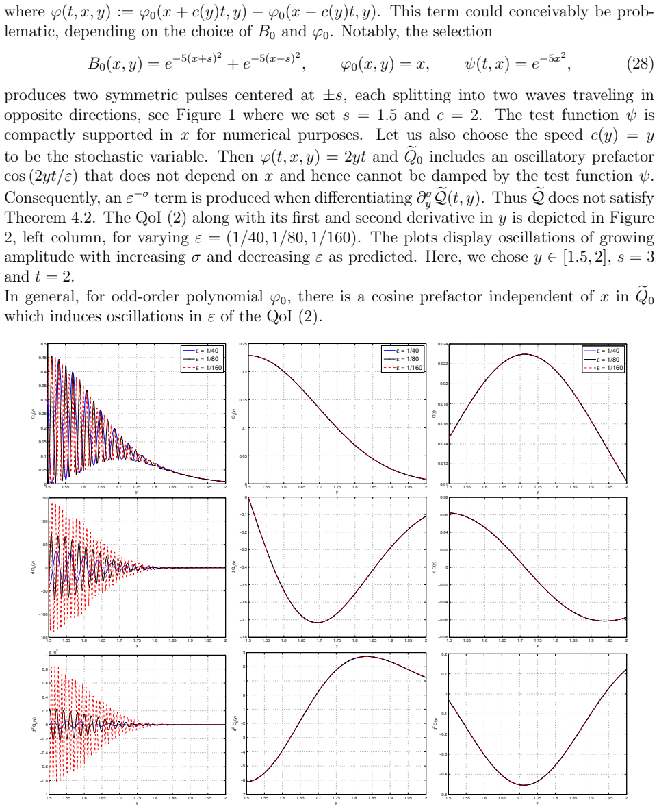
Summary. The paper studies the stochastic regularity of quadratic observables of high-frequency solutions to the scalar wave equation with random coefficients and initial data, in the regime where the wavelength ε is small. The quantities of interest have the form ε^{2(p+|α|)}∫∫ g |∂_t^p ∂_x^α u|^2 ψ dx dt, and the solution u is approximated by a sum of two Gaussian-beam modes. The main result, Theorem 5.2, states that under hypotheses (A1)–(A5) and with an admissible beam cutoff width η, every mixed derivative of the Gaussian-beam QoI Q^{GB}_{p,α}(y) with respect to the parameters y is bounded uniformly in ε on compact parameter sets. The proof splits the QoI into same-mode contributions, handled by the one-mode theorem (Theorem 4.2), and a cross term. The cross term is controlled by a non-stationary phase argument in time: Proposition 5.5 shows that the phase derivative |∂_t ϑ_k| is bounded below by a positive constant on the relevant spatial region, and Lemma 5.3 converts this into arbitrarily high powers of ε. Numerical examples in Sections 5.1 and 5.4 illustrate the difference between the oscillatory space-only QoI and the non-oscillatory time-averaged QoI.

Significance. The result is a substantive extension of the authors' earlier one-mode result [23] to two-mode Gaussian-beam solutions and to observables involving higher derivatives of the wave field. If correct, it provides a theoretical justification for stochastic collocation and stochastic Galerkin methods applied to Gaussian-beam approximations in the high-frequency regime, which is the regime where direct numerical simulation is prohibitively expensive. The proof is careful and largely explicit: the ε-power bookkeeping is tracked through the non-stationary phase lemma, the constants are kept visible, and the assumptions (A1)–(A5) are used in an essential way. The numerical examples are helpful and confirm the qualitative difference between space-only and space-time averaged observables. The paper relies on published prior results for the one-mode input, which is acceptable but makes the paper not fully self-contained.

minor comments (5)

[Section 5.3, Eq. (38)] There is a sign error in the displayed formula for ∂_t ϑ_k. Using (11), ∂_t q^± = ± c(q^±)p^±/|p^±|, so the right-hand side should read +c(q^-,y)|p^-| + c(q^+,y)|p^+| + R_k, not −c(q^-,y)|p^-| − c(q^+,y)|p^+| + R_k. The subsequent lower bound in Proposition 5.5 uses the positive sum, so the display should be corrected to match the argument.
[Section 5.3, after Eq. (41)] The support statement for g_{ℓmjσ} := f_{ℓmjσ} ψ g_1 says supp g_{ℓmjσ}(t,·) ⊂ Σ_{μ/2}, but g_1 = ϱ_μ(x−q^+)ϱ_μ(x−q^-) is supported only in Σ_μ (since ϱ_μ has support in B_{2μ}), not in Σ_{μ/2}. The correct statement is supp g_{ℓmjσ}(t,·) ⊂ Σ_μ, and the argument still works because Proposition 5.5 provides the lower bound on Σ_μ.
[Section 4.2 and Appendix] Theorem 4.6, which is the load-bearing input for the one-mode result, is not proved in this paper: the appendix invokes [23, Lemma 5] and [23, Lemma 6] and says the rest of the proof of [23, Theorem 1] can be used as is. Proposition 4.1 is also delegated to [22] and [23]. Since Theorem 5.2 depends on these results, the paper would be easier to verify if the authors stated explicitly which lemmas from [23] are reused and confirmed that they apply under the present slightly generalized hypotheses (t-dependent ψ, compact subsets of an open set Γ).
[Theorems 4.2 and 5.2] There are small notation inconsistencies in the statements: the spatial multi-index is written as α ∈ N_0^N in places where it should be α ∈ N_0^n, and the parameter derivative multi-index is σ ∈ N_0^N. Also, Eq. (5) in the introduction writes ∂^σ Q/∂y^σ twice.
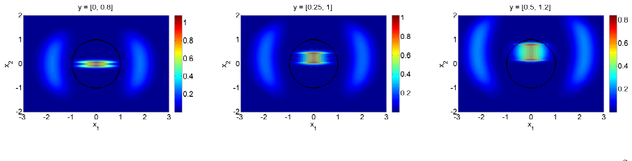
[Sections 5.1 and 5.4] The illustrative examples use Gaussian initial data with unbounded support and, in Section 5.4, a non-smooth phase containing |x_1|, so they do not satisfy assumptions (A2) and (A3). This is acceptable for heuristic illustration, but the text should note explicitly that these examples lie outside the theorem's hypotheses.

Circularity Check

0 steps flagged · score 0.0 of 10

No circularity found; the two-mode bound is proved from the stated assumptions, with the one-mode estimate delegated to a published prior proof.

full rationale

The derivation of Theorem 5.2 is not circular. The two-mode cross term Q3 is estimated directly in Section 5.3: Proposition 5.5 proves |∂tϑk| ≥ ν using Hamiltonian conservation from (11) together with (A1) and (A3) and a small cutoff μ, and the subsequent partition-of-unity argument combines the non-stationary phase lemma (Lemma 5.3) with the exponential decay of Im ϑk from (39). None of these steps assumes the desired y-derivative bound. The one-mode contributions Q1 and Q2 are delegated to Theorem 4.2, whose proof relies on Theorem 4.6; Theorem 4.6 is proved in Appendix A with the comment 'The rest of the proof of [23, Theorem 1] can be used as it is' and uses [23, Lemmas 5 and 6]. Although [23] is a self-citation, it is a published theorem with an independent proof, and the present argument does not assume Theorem 5.2 in proving it. The admissibility of η in Definition 2 is a phase-decay condition proved in Proposition 5.1 from (A1)-(A3), not the target estimate. No fitted parameters or data enter the proof. Thus no step reduces to its inputs by construction; the only weakness is a verifiability burden from delegating the one-mode estimates to earlier work by the same authors.

Assumptions & free parameters 2 free parameters · 6 assumptions · 0 invented entities

The central claim rests on explicit smoothness and compact-support assumptions (A1-A3, A5), an admissibility property of Gaussian beam phases inherited from prior work, and the classical non-stationary phase lemma. No new physical entities are introduced, and the only hand-chosen parameters are the proof cutoffs η and μ, which are existential and not fitted to observations.

free parameters (2)

Admissible Gaussian beam cutoff width η = exists but not numerically specified
Chosen in Propositions 4.1 and 5.1 so that Im Φ ≥ δ|x|^2 on B_{2η}; the proof of Theorems 4.2 and 5.2 holds for any sufficiently small η, and all final constants depend on η.
Secondary cutoff μ = not specified, chosen small enough
Chosen in Proposition 5.5 and in the proof of Theorem 5.2 to make the cross-term phase derivative bounded below; the final constant C_σ depends on μ.

assumptions (6)

domain assumption A1: c ∈ C^∞(R^n × Γ), 0 < c_min ≤ c ≤ c_max < ∞, uniformly bounded derivatives in x and y.
Stated in Section 2; needed for well-posed rays and for smooth dependence of the Gaussian beam coefficients on y.
domain assumption A2: Initial amplitudes B_0 and B_1 are smooth and compactly supported uniformly in y.
Stated in Section 2; ensures the beam superposition is a finite integral over K_0 and all beam coefficients have compact support in z.
domain assumption A3: Initial phase φ_0 is smooth and |∇φ_0| > 0 for all x ∈ R^n, y ∈ Γ.
Stated in Section 2; guarantees p^±(0) = ∇φ_0 ≠ 0, so the Hamiltonian c(q)|p| is conserved with a positive lower bound γ > 0, which is the crux of Proposition 5.5.
domain assumption A5: Test function ψ ∈ C_c^∞(R × R^n) with supp ψ ⊂ [0,T] × K_1.
Stated in Section 2; gives the space-time locality used in the non-stationary phase argument and reduces the infinite time integral to [0,T].
domain assumption Proposition 4.1: For a small enough cutoff width, Im Φ_k ≥ δ|x|^2 on the beam cutoff ball.
Restated from [23, Prop. 1] with proof in [22]; this admissibility controls the Gaussian decay of beams and is the basis for the weighted estimates.
standard math Lemma 5.3: Non-stationary phase lemma with explicit constants.
Classical result from Hörmander [13]; stated to keep track of the dependence of the constant on the phase when applied to the cross-term integral.

how reviews work

0 comments

Cite this review

Pith. "Pith review of Stochastic regularity of general quadratic observables of high frequency waves." pith.science (2026). https://pith.science/paper/3NERD5QC

@misc{pith2026190807472,
  author       = {Pith},
  title        = {Pith review of: Stochastic regularity of general quadratic observables of high frequency waves},
  year         = {2026},
  howpublished = {\url{https://pith.science/paper/3NERD5QC}},
  note         = {Machine review of arXiv:1908.07472}
}

abstract

We consider the wave equation with uncertain initial data and medium, when the wavelength $\varepsilon$ of the solution is short compared to the distance traveled by the wave. We are interested in the statistics for quantities of interest (QoI), defined as functionals of the wave solution, given the probability distributions of the uncertain parameters in the wave equation. Fast methods to compute this statistics require considerable smoothness in the mapping from parameters to the QoI, which is typically not present in the high frequency case, as the oscillations on the $\varepsilon$ scale in the wave field is inherited by the QoIs. The main contribution of this work is to identify certain non-oscillatory quadratic QoIs and show $\varepsilon$-independent estimates for the derivatives of the QoI with respect to the parameters, when the wave solution is replaced by a Gaussian beam approximation.

Figures

Figures reproduced from arXiv: 1908.07472 by the authors.

**Figure 1.** d’Alembert solution with initial data (25) and (28). 5 Two-mode quantity of interest Let us consider a wave composed of both forward and backward propagating modes as defined in (15). In this case, Theorem 4.2 for the QoI (17) is no longer necessarily true. In fact, Qep,α GB can be highly oscillatory. We will therefore have to look at a slightly different QoI where the averaging is also done in time, not just in spa… view at source ↗

**Figure 2.** Left column: QoI (2) with ϕ0(x, y) = x, and its first and second derivative in y. Central column: QoI (2) with ϕ0(x, y) = x 2 . Right column: QoI (4) with ϕ0(x, y) = x. Note that when ϕ0 is an even-order polynomial in x, the QoI is not oscillatory for the example 15 [PITH_FULL_IMAGE:figures/full_fig_p015_2.png] view at source ↗

**Figure 3.** The modulus of the GB solution |u1(t, x, y)| for ε = 1/60 and ϕ0(x, y) = |x1| + (x2 − y1) 2 , at time t = 1, for various y. The circle denotes the support of the test function ψ. 0 0.2 0.4 0.6 0.8 1 0.01 0.02 0.03 0.04 0.05 0.06 r Q(r) ε = 1/20 ε = 1/40 ε = 1/80 0 0.2 0.4 0.6 0.8 1 0.01 0.02 0.03 0.04 0.05 0.06 0.07 r Q(r) 0 0.2 0.4 0.6 0.8 1 1.5 2 2.5 3 3.5 4 4.5 5 5.5 x 10−3 r Q(r) 0 0.2 0.4 0.6 0.8 1 −0.1 −0.08 −… view at source ↗

Figures from the paper (2 more)

**Figure 4.** Figure 4: Left column: QeGB and its first and second derivatives for one-mode solution. Central column: QeGB and its first and second derivatives for two-mode solution. Right column: QGB and its first and second derivatives for two-mode solution. Let us now consider the same set…

**Figure 5.** Figure 5: The modulus of the GB solution |u1(t, x, y)| for ε = 1/60 and ϕ0(x, y) = x1 + (x2 − y1) 2 at time t = 1, for various y. The circle denotes the support of the test function ψ. Three realizations of |u1(t, x, y)| at t = 1 are shown in [PITH_FULL_IMAGE:figures/full_fig_p…

Discussion (0). Continue with ORCID to comment.

Reference graph

Works this paper leans on

34 extracted references · 32 canonical work pages

[23]

Malenová, M

G. Malenová, M. Motamed, and O. Runborg. Stochastic regularity of a quadratic ob- servable of high-frequency waves.Res. Math. Sci., 4(1):1–23, 2017. 28

work page 2017
[22]

Malenová.Uncertainty quantiﬁcation for high frequency waves

G. Malenová.Uncertainty quantiﬁcation for high frequency waves. Licentite thesis, KTH Royal Institute of Technology, 2016

work page 2016
[1]

Babuska, F

I. Babuska, F. Nobile, and R. Tempone. A stochastic collocation method for elliptic partial diﬀerential equations with random input data.SIAM Rev., 52:317–355, 2010

work page 2010
[2]

Babuska, R

I. Babuska, R. Tempone, and G. E. Zouraris. Solving elliptic boundary value problems with uncertain coeﬃcients by the ﬁnite element method: the stochastic formulation. Comput. Method. Appl. M., 194:1251–1294, 2005

work page 2005
[3]

I. M. Babuska, F. Nobile, and R. Tempone. A stochastic collocation method for elliptic partial diﬀerential equations with random input data.SIAM J. Numer. Anal., 45:1005– 1034, 2007

work page 2007
[4]

Bamberger, B

A. Bamberger, B. Engquist, L. Halpern, and P. Joly. Parabolic wave equation approxi- mations in heterogeneous media.SIAM J. Appl. Math., 48(1):99–128, 1988

work page 1988
[5]

Bungartz and M

H.-J. Bungartz and M. Griebel. Sparse grids.Acta Numer., 13:147–269, 2004

work page 2004
[6]

Cervený, M

V. Cervený, M. M. Popov, and I. Pšenčík. Computation of wave ﬁelds in inhomogeneous media — Gaussian beam approach.Geophys. J. R. Astr. Soc., 70:109–128, 1982

work page 1982

Show all 34 references

[7]

Cohen, R

A. Cohen, R. Devore, and C. Schwab. Analytic regularity and polynomial approximation of parametric and stochastic elliptic PDEs.Anal. Appl., 9:11–47, 2011

2011
[8]

Engquist and O

B. Engquist and O. Runborg. Computational high frequency wave propagation.Acta Numer., 12:181–266, 2003

2003
[9]

G. S. Fishman.Monte Carlo: Concepts, Algorithms, and Applications. Springer- Verlag, New York, 1996. 27

1996
[10]

Stochastic ﬁnite elements: A spectral approach

R.G.GhanemandP.D.Spanos. Stochastic ﬁnite elements: A spectral approach. Springer, New York, 1991

1991
[11]

Griebel and S

M. Griebel and S. Knapek. Optimized general sparse grid approximation spaces for operator equations. Math. Comp., 78:2223–2257, 2009

2009
[12]

Robert J Hansen.Seismic design for nuclear power plants.The MIT Press, Cambridge, 1970

1970
[13]

Hörmander

L. Hörmander. The Analysis of Linear Partial Diﬀerential Operators I: Distribution Theory and Fourier Analysis. Springer-Verlag, 1983

1983
[14]

Jin, J.-G

S. Jin, J.-G. Liu, and Z. Ma. Uniform spectral convergence of the stochastic Galerkin method for the linear transport equations with random inputs in diﬀusive regime and a micro-macro decomposition based asymptotic preserving method.Res. Math. Sci., 4(15), 2017

2017
[15]

S. Jin, L. Liu, G. Russo, and Z. Zhou. Gaussian wave packet transform based numerical scheme for the semi-classical Schrödinger equation with random inputs. Technical report, arXiv:1903.08740 [math.NA], 2019

1903 arXiv
[16]

Jin and Y

S. Jin and Y. Zhu. Hypocoercivity and uniform regularity for the Vlasov-Poisson Fokker– Planck system with uncertainty and multiple scales.SIAM J. Math. Anal., 50:1790–1816, 2018

2018
[17]

J. Li, Z. Fang, and G. Lin. Regularity analysis of metamaterial Maxwell’s equations with random coeﬃcients and initial conditions.Comput. Method. Appl. M., 335:24–51, 2018

2018
[18]

Li and L

Q. Li and L. Wang. Uniform regularity for linear kinetic equations with random in- put based on hypocoercivity.SIAM/ASA J. Uncertainty Quantiﬁcation, 5(1):1193–1219, 2017

2017
[19]

H. Liu, O. Runborg, and N. M. Tanushev. Error estimates for Gaussian beam superpo- sitions. Math. Comp., 82:919–952, 2013

2013
[20]

H. Liu, O. Runborg, and N. M. Tanushev. Sobolev and max norm error estimates for Gaussian beam superpositions.Commun. Math. Sci., 14(7):2037–2072, 2016

2016
[21]

Liu and S

L. Liu and S. Jin. Hypocoercivity based sensitivity analysis and spectral convergence of the stochastic Galerkin approximation to collisional kinetic equations with multiple scales and random inputs.Multiscale Model. Simul., 16(3):1085–1114, 2017

2017
[24]

Malenová, M

G. Malenová, M. Motamed, O. Runborg, and R. Tempone. A sparse stochastic collo- cation technique for high-frequency wave propagation with uncertainty.SIAM/ASA J. Uncertainty Quantiﬁcation, 4(1):1084–1110, 2016

2016
[25]

Motamed, F

M. Motamed, F. Nobile, and R. Tempone. A stochastic collocation method for the second order wave equation with a discontinuous random speed.Num. Math., 123(3):495–546, 2013

2013
[26]

Nobile and R

F. Nobile and R. Tempone. Analysis and implementation issues for the numerical ap- proximation of parabolic equations with random coeﬃcients.IJNME, 80:979–1006, 2009

2009
[27]

Nobile, R

F. Nobile, R. Tempone, and C. G. Webster. A sparse grid stochastic collocation method for partial diﬀerential equations with random input data. SIAM J. Numer. Anal., 46:2309–2345, 2008

2008
[28]

J. Ralston. Gaussian beams and the propagation of singularities. Studies in partial diﬀerential equations, 23:206–248, 1982

1982
[29]

O. Runborg. Mathematical models and numerical methods for high frequency waves. Commun. Comput. Phys., 2:827–880, 2007

2007
[30]

R. W. Shu and S. Jin. Uniform regularity in the random space and spectral accuracy of the stochastic Galerkin method for a kinetic-ﬂuid two-phase ﬂow model with random initial inputs in the light particle regime.M2AN, 52:1651–1678, 2018

2018
[31]

N. M. Tanushev. Superpositions and higher order Gaussian beams.Commun. Math. Sci., 6(2):449–475, 2008

2008
[32]

R. A. Todor and C. Schwab. Convergence rates for sparse chaos approximations of elliptic problems with stochastic coeﬃcients.IMA J. Numer. Anal., 27:232–261, 2007

2007
[33]

Xiu and J

D. Xiu and J. S. Hesthaven. High-order collocation methods for diﬀerential equations with random inputs.SIAM J. Sci. Comput., 27:1118–1139, 2005

2005
[34]

Xiu and G

D. Xiu and G. E. Karniadakis. Modeling uncertainty in steady state diﬀusion problems via generalized polynomial chaos.Comput. Method. Appl. M., 191:4927–4948, 2002. 29

2002

Pith tools

Reviewed August 14, 2026 · model on record in the stance chip above.

[1] [23]

Malenová, M

G. Malenová, M. Motamed, and O. Runborg. Stochastic regularity of a quadratic ob- servable of high-frequency waves.Res. Math. Sci., 4(1):1–23, 2017. 28

work page 2017

[2] [22]

Malenová.Uncertainty quantiﬁcation for high frequency waves

G. Malenová.Uncertainty quantiﬁcation for high frequency waves. Licentite thesis, KTH Royal Institute of Technology, 2016

work page 2016

[3] [1]

Babuska, F

I. Babuska, F. Nobile, and R. Tempone. A stochastic collocation method for elliptic partial diﬀerential equations with random input data.SIAM Rev., 52:317–355, 2010

work page 2010

[4] [2]

Babuska, R

I. Babuska, R. Tempone, and G. E. Zouraris. Solving elliptic boundary value problems with uncertain coeﬃcients by the ﬁnite element method: the stochastic formulation. Comput. Method. Appl. M., 194:1251–1294, 2005

work page 2005

[5] [3]

I. M. Babuska, F. Nobile, and R. Tempone. A stochastic collocation method for elliptic partial diﬀerential equations with random input data.SIAM J. Numer. Anal., 45:1005– 1034, 2007

work page 2007

[6] [4]

Bamberger, B

A. Bamberger, B. Engquist, L. Halpern, and P. Joly. Parabolic wave equation approxi- mations in heterogeneous media.SIAM J. Appl. Math., 48(1):99–128, 1988

work page 1988

[7] [5]

Bungartz and M

H.-J. Bungartz and M. Griebel. Sparse grids.Acta Numer., 13:147–269, 2004

work page 2004

[8] [6]

Cervený, M

V. Cervený, M. M. Popov, and I. Pšenčík. Computation of wave ﬁelds in inhomogeneous media — Gaussian beam approach.Geophys. J. R. Astr. Soc., 70:109–128, 1982

work page 1982