REVIEW 3 major objections 4 minor 123 references
Modeling UV Radiation Feedback from Massive Stars: III. Escape of Radiation from Star-forming Giant Molecular Clouds
T0 review · 3 major / 4 minor · reviewed 2026-08-14 · deepseek-v4-flash
Pith's one-line read Turbulence, not mean dust, controls how much UV light escapes star-forming clouds.
desk verdict Solid simulation paper with a new optical-depth PDF framework; the headline accuracy claims are in-sample and absolute escape fractions rest on a flagged subgrid assumption, so treat the quantitative range as indicative rather than final. read the letter →
The pith
A machine-rendered reading of the paper's core claim, the machinery that carries it, and where it could break.
The reading
What carries the argument
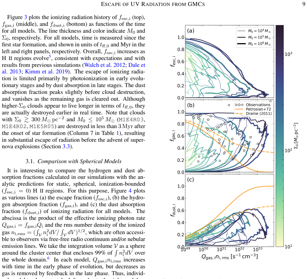
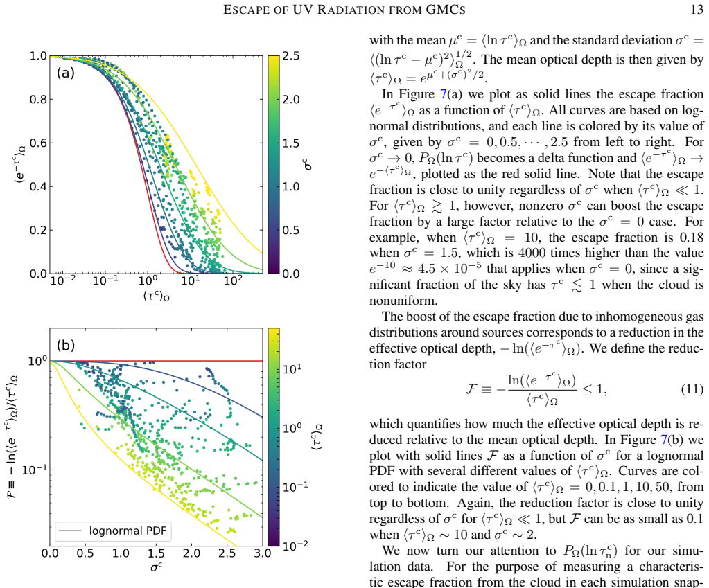
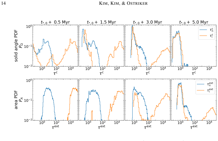
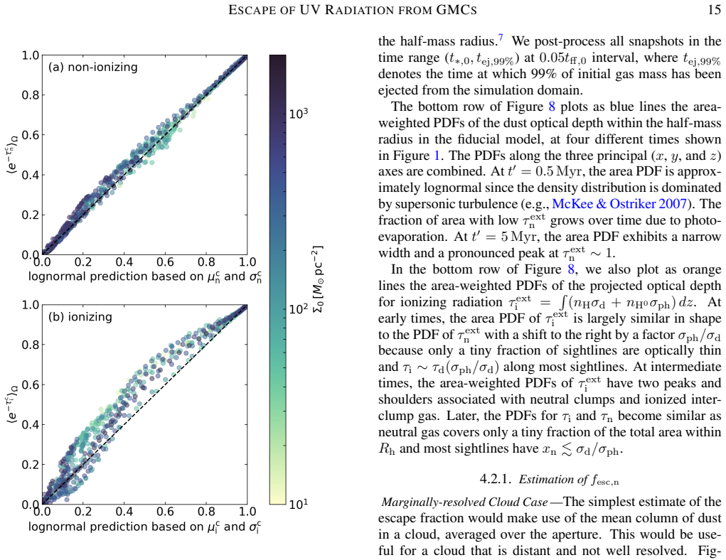
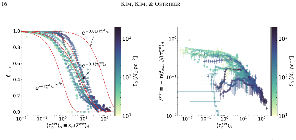
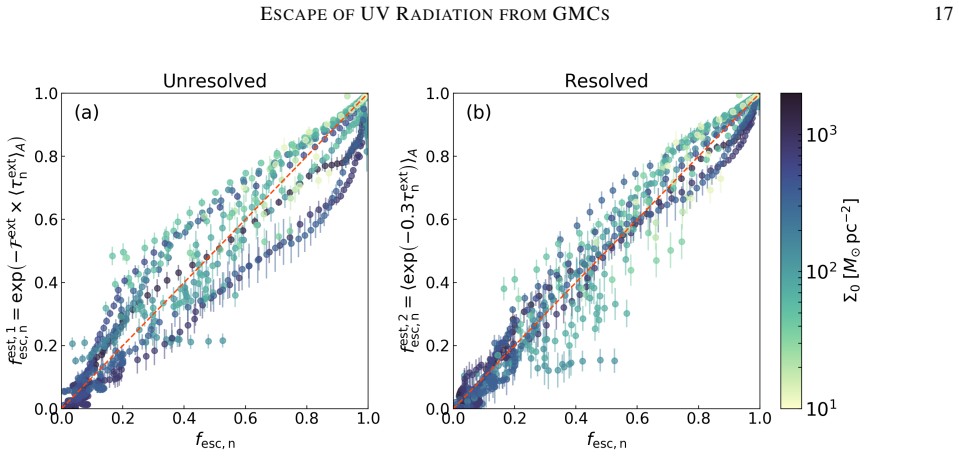
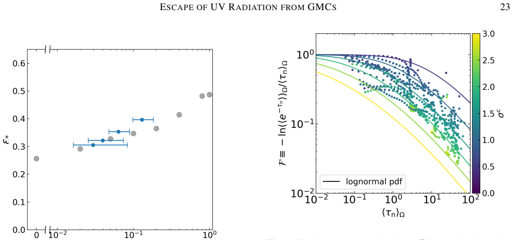
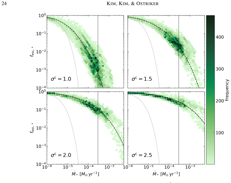
The central object is the optical-depth probability distribution function, $P(\ln\tau)$, measured either as a solid-angle-weighted distribution from the source position or as an area-weighted distribution projected on the sky. The escape fraction for non-ionizing radiation is the solid-angle average $\langle e^{-\tau}\rangle_\Omega$, which by Jensen's inequality is always at least $e^{-\langle\tau\rangle}$; a lognormal fit with measured mean and width reproduces the true escape fractions within 7% (non-ionizing) and 20% (ionizing). For observers, the paper introduces a reduction factor $F = -\ln(f_{\rm esc})/\langle \tau\rangle$ and two estimators: $f_{\rm esc,n} = \exp(-\eta_1 \langle \tau_{\rm ext}\rangle_A)$ with $\eta_1 = 0.56/(1 + 1.25\langle \tau_{\rm ext}\rangle_A^{0.48})$ for marginally resolved clouds, and $f_{\rm esc,n} = \langle \exp(-0.3\, \tau_{\rm ext})\rangle_A$ for resolved clouds.
What would settle it
Measure the projected dust optical depth distribution around a young embedded cluster in a resolved giant molecular cloud (for example, via near-infrared extinction) and compare the predicted $f_{\rm esc,n} = \langle \exp(-0.3\, \tau_{\rm ext})\rangle_A$ with the escape fraction inferred by comparing the cluster's Hα or free-free luminosity to the ionizing photon rate expected from its stellar content; a systematic discrepancy larger than about 20% would falsify the calibration.
Extended reading notes
Core claim
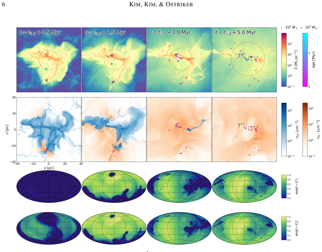
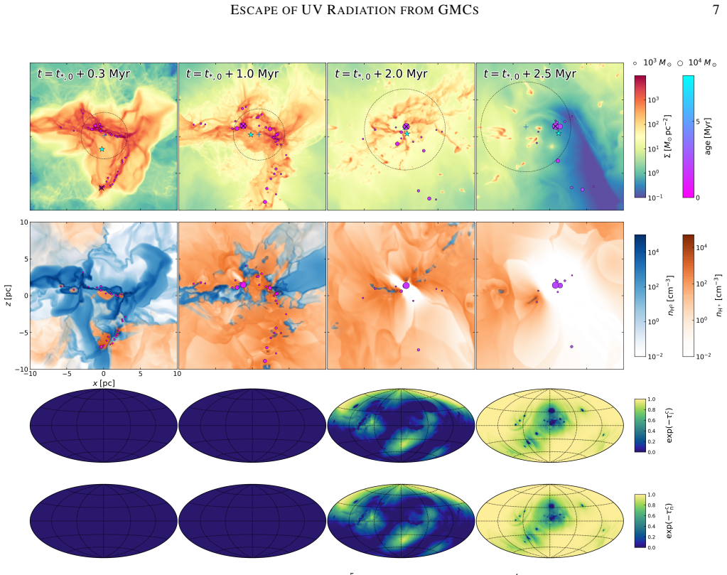
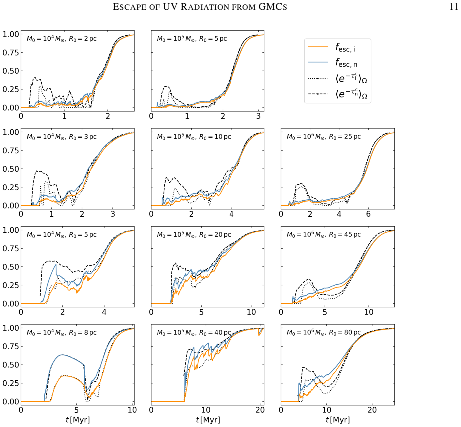
On the paper's own terms, the central discovery is that the escape fraction of both ionizing and non-ionizing radiation from a star-forming GMC is largely set by the solid-angle distribution of dust optical depth as seen from the stellar luminosity center: escape increases with smaller mean $\langle \tau\rangle$ and larger dispersion $\sigma$, and exceeds the one-zone estimate $e^{-\langle \tau\rangle}$ by up to three orders of magnitude because turbulence produces a wide lognormal-like tail of low-opacity sightlines. The simulations show that once H II regions break out, photons escape through the same fully ionized low-density channels, so $f_{\rm esc,n} \approx f_{\rm esc,i}$ at late times even though the two frequency bins have very different physical opacities; dust becomes the dominant absorber of ionizing photons. As a practical corollary, the escape fraction can be recovered from externally projected dust optical depth using two simple calibrations, accurate to about 20% in the models.
Load-bearing premise
The simulations assume that every photon emitted by a star particle leaves the unresolved control volume around it without any absorption ($f_{\rm esc,*} = 1$); if the accreting gas right around the stars absorbs a significant part of the ultraviolet radiation, all quoted cloud-scale escape fractions and the calibration of the estimators are systematically too high.
Editorial extensions
If this is right
- Star formation rates in individual clouds inferred from dust-corrected Hα or ultraviolet emission will be underestimated unless the escaped photon fraction is added back; the paper's estimators provide a correction from the same dust maps used for extinction.
- The similarity of $f_{\rm esc,i}$ and $f_{\rm esc,n}$ at late times implies that diffuse ionized gas on galactic scales can be powered by Lyman-continuum leakage from GMCs without requiring a separate population of exceptionally leaky H II regions.
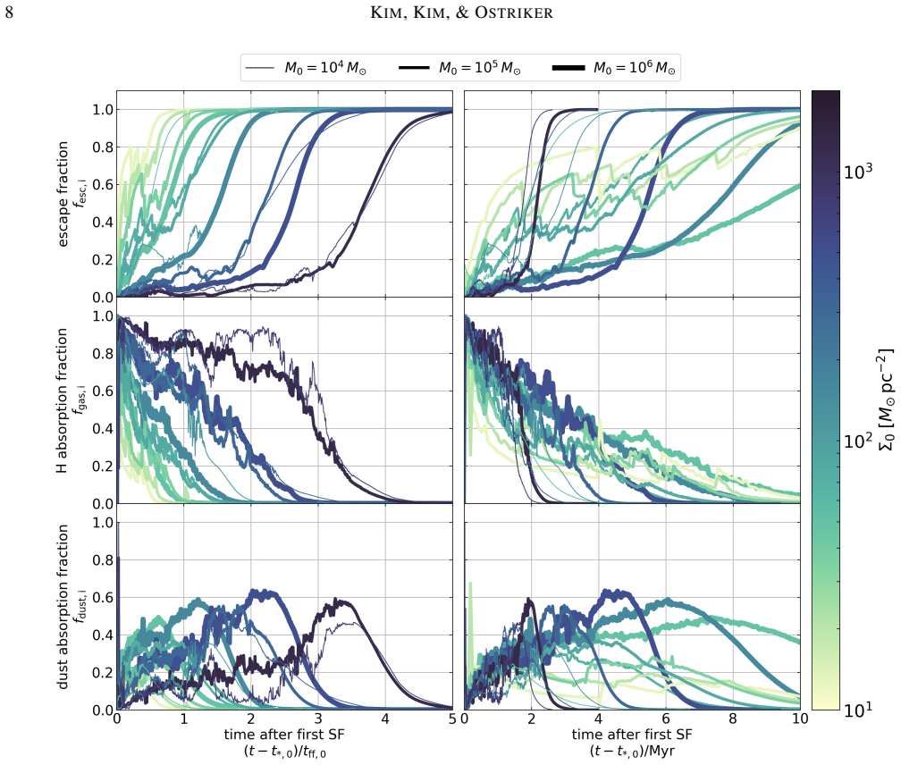
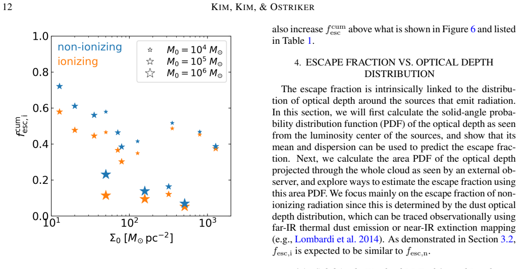
- The cumulative escape fraction before the first supernova ranges from a few percent to roughly 50%, with compact clouds of high surface density, which are destroyed within 3 Myr, contributing the highest fractions; massive $10^6\,M_\odot$ clouds leak very little before supernovae.
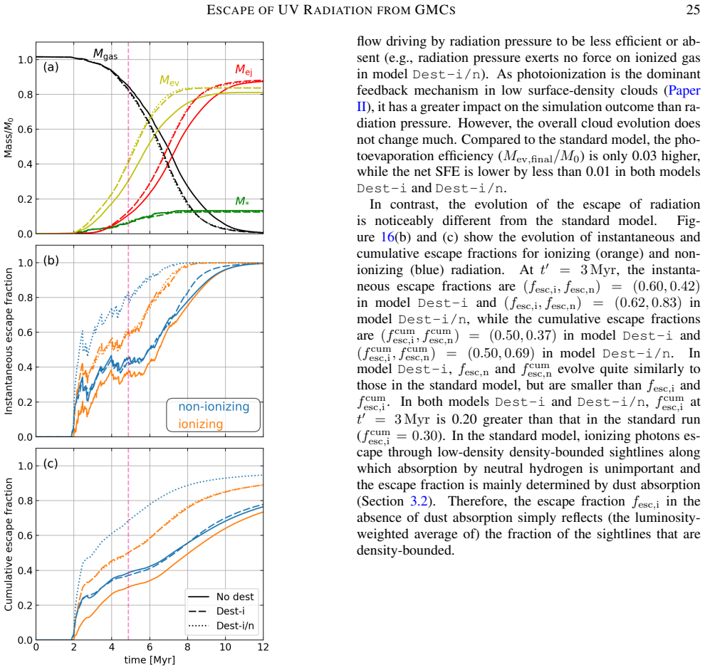
- If dust is destroyed in ionized gas, the ionizing cumulative escape fraction for the fiducial cloud rises by about 0.2, bounding the role of grain destruction in boosting photon escape.
Reading between the lines
- A testable consequence not drawn in the paper: the same two estimators should work on observed column-density PDFs of Galactic clouds, provided the dust opacity per hydrogen is known; the scatter in the paper's Figure 12 predicts that the direct area-averaged estimator ($\eta = 0.3$) will outperform the mean-based one for clouds with resolved column-density maps.
- The reduction-factor framework suggests a dimensionless diagnostic: for any star-forming cloud, measuring $\tau_{\rm ext}$ along many sightlines and plotting $F$ versus $\langle \tau\rangle$ should collapse onto the simulation band if turbulence and feedback are the main sources of opacity spread.
- Extending beyond the paper's pre-supernova horizon, the steep drop in ionizing photon production after 3 Myr implies that supernovae may clear remaining gas but not add many escaping Lyman-continuum photons, shifting the epoch of maximum leakage earlier in the cloud lifetime.
- The subgrid escape assumption $f_{\rm esc,*} = 1$ is the paper's stated caveat; if accreting flows near sink particles absorb photons, the quoted cumulative escape fractions are upper limits, and the calibration constants $\eta_1$ and $\eta_2$ would need recalibration toward smaller escape.
Signed reviews
Editorial analysis
A structured set of objections, weighed in public.
Referee Report
Summary. This paper presents radiation-hydrodynamic simulations of star cluster formation in turbulent giant molecular clouds, covering two orders of magnitude in cloud mass and surface density, and analyzes the escape fractions of ionizing (LyC) and non-ionizing (FUV) radiation. The authors find that escape fractions increase with time as H II regions break out, that cumulative escape fractions before the first supernova range from 5% to 58% for ionizing and 7% to 72% for non-ionizing radiation, and that the escape fraction is largely determined by the mean and width of the optical depth distribution rather than the naive exp(-<tau>) estimate. They propose two observationally oriented estimators for fesc,n based on the area-averaged dust optical depth or its resolved distribution, claiming accuracy within about 20%.
Significance. If the results hold, this is a valuable systematic numerical study: it spans a wider parameter space than most prior work, treats both ionizing and non-ionizing radiation consistently, and provides a physically transparent reduction of the escape problem to optical-depth PDF moments. The two proposed estimators are potentially useful for converting observed dust column maps into escape-fraction corrections for star formation indicators. The paper is also honest in its treatment of caveats: Appendices A and B explicitly address subgrid escape, dust destruction, and resolution effects, and the authors state in Section 5.2.5 that the cloud-scale escape fraction may be overestimated because of the fesc,* = 1 assumption. These features make the work a substantive contribution to the theory of UV feedback and photon escape from star-forming clouds.
major comments (3)
- [Section 2.2 and Section 5.2.5] The assumption fesc,* = 1, namely that all photons emitted by a sink particle emerge from the 3^3-cell control volume without subgrid absorption, is load-bearing for the two central quantitative claims: the cumulative escape fraction range (Table 1, Columns 9 and 12) and the calibration of the estimators in Equations (12) and (13). The authors explicitly concede in Section 5.2.5 that the cloud-scale escape fraction may be an overestimate due to this assumption. However, the mitigation offered in Appendix A does not directly address the problem: the experiments in Section A.3 vary fesc,* only in radiation-pressure-only models and report changes in the net star formation efficiency (Figure 13), not changes in fesc,n or fesc,i in the photoionization-dominated models that set the headline results. The statement in Section 5.2.1 that effects on fesc are 'relatively modest' is therefore not supported by the presented tests. This is a specific, fixable gap: the authors should either run the fesc,* variation for photoionization-dominated clouds and report the resulting escape fractions, or visibly weaken the quantitative claims about the absolute escape fraction range.
- [Section 4.2.1, Equations (12) and (13)] The stated accuracy of the two estimators ('within ~20%') is measured on the same simulation snapshots used to fit the parameters a = 1.25, b = 0.48, and eta2 = 0.30. This is an in-sample fit, so the 20% figure is not a predictive accuracy; it is a measure of the fit's residuals. For the claim that these methods can estimate observed escape fractions, the manuscript should provide some out-of-sample assessment (e.g., cross-validation across models or across time, or a held-out subset of the snapshot data). As written, a reader cannot distinguish the estimator's intrinsic scatter from the flexibility of the adopted functional form.
- [Section 2.2 and Section 4.1] The use of a single luminosity center to characterize the optical-depth PDF (Section 4.1) is systematically inaccurate in the early embedded phase when sources are clustered in a few widely separated regions; the authors acknowledge this in the text. This is not a fatal flaw because the quantitative escape fractions themselves are directly measured from the ray tracing, but it should be kept in mind when interpreting the PDF-based estimators: the claimed agreement between the luminosity-center reconstruction and the true escape fraction is demonstrated only for the later, more centrally concentrated phases. A quantitative statement of the early-phase discrepancy (how much larger the luminosity-center estimate is) would strengthen the paper.
minor comments (4)
- [Section 3.1] There is a typo: 'Galctic H II regions' should be 'Galactic H II regions'.
- [Appendix B, Figure 16 caption] The caption of Figure 16 lists 'Dest-i' and 'Dest-i/n' but the text in Section 5.2.4 refers to 'complete destruction' cases; consider defining the abbreviations more explicitly at first use.
- [Figure 15 caption] The caption appears to have a typo: it lists sigma_c = 1.0, 2.0, 2.0, 2.5, while the text discusses sigma_c = 1.0, 1.5, 2.0, 2.5.
- [Section 5.2.5] The phrase 'could further increase' appears in the discussion of stellar winds and outflows; consider 'could also increase' to avoid the implication that the previously discussed subgrid absorption already increases porosity.
Circularity Check
The claimed ~20% estimator accuracy is in-sample calibration: the constants in Equations (12) and (13) are least-squares fitted to the same simulation snapshots on which the 'prediction' is then evaluated.
-
fitted input called prediction
[Section 4.2.1, Equations (12) and (13), Figures 10-12]
"We perform a least square fit to find parameters a = 1.25, b = 0.48 that minimize the sum of squared errors ((fesc,n - fest,1esc,n)^2) compared to our simulation results. ... This estimator predicts fesc,n within ~20%. ... We also adopt the constant value of eta2 for all snapshots and find that eta2 = 0.30 minimizes the sum of the square of the differences (fest,2esc,n - fesc,n)^2. Figure 12(b) compares fest,2esc,n with the actual escape fraction, again showing that this method predicts fesc,n within 20%."
The parameters a, b, and eta2 that define estimators (12) and (13) are obtained by least-squares minimization against the full set of simulation snapshots from all models, and the claimed 'predicts within ~20%' accuracy is then demonstrated by plotting those same estimators against those same snapshots in Figure 12. Thus the quoted 20% is the in-sample residual of a fit, not an out-of-sample prediction. By construction, the fitted curve minimizes the very squared-error statistic that is used to support the accuracy claim, so the predictive statement reduces to the calibration procedure unless an independent test set, cross-validation, or external data were used, which the paper does not provide.
full rationale
The central physical derivation is not circular: the escape fractions fesc,i and fesc,n are directly measured from the adaptive ray-tracing simulations, the optical-depth PDFs are computed independently from the density fields, and the inequality in Equation (9) is a general mathematical statement. The finding that fesc increases with smaller mean optical depth and larger dispersion is a genuine analysis of simulation data, not an input assumption. The lognormal approximation is also tested against the raw PDFs rather than assumed to be identical to them. The main circularity is confined to the estimator section: the paper fits the free constants of Equations (12) and (13) to all simulation snapshots and then calls the resulting agreement a prediction within 20%. This is in-sample by construction. The paper's self-citations to Paper I and Paper II are methodological provenance for the code and simulation suite, not load-bearing citations that smuggle in the escape-fraction result. The limitation flagged in Section 5.2.5 that the subgrid assumption fesc,* = 1 may make the cloud-scale escape fractions overestimates is an acknowledged modeling caveat, not a circular step; similarly, Appendix A tests subgrid escape effects on SFE rather than on fesc, which is a support gap but not circularity.
Assumptions & free parameters
free parameters (3)
- eta1 normalization parameter a =
1.25
- eta1 exponent parameter b =
0.48
- eta2 correction factor =
0.30
assumptions (7)
- domain assumption The gas temperature is fixed at 20 K when fully neutral and 8000 K when fully ionized, with smooth interpolation based on neutral fraction; cooling time is assumed short.
- domain assumption Photons emitted by sink particles escape their 3^3-cell control volume without absorption (fesc,* = 1).
- domain assumption Constant dust absorption cross section per hydrogen, sigma_d = 1.17e-21 cm^2, applies to both ionizing and non-ionizing radiation; dust scattering is neglected.
- standard math The solid-angle optical-depth distribution P(ln tau) can be approximated as lognormal to relate the mean and width to the escape fraction.
- domain assumption The initial cloud is a uniform-density sphere with virial parameter alpha_vir,0 = 2 and a decaying turbulent velocity field, with no magnetic fields or external pressure.
- domain assumption Stellar UV luminosity and ionizing photon rate scale with cluster mass via median IMF fits, without time evolution during the 3 Myr period.
- standard math Jensen's inequality for the exponential of optical depth: <exp(-tau)> >= exp(-<tau>).
Cite this review
Pith. "Pith review of Modeling UV Radiation Feedback from Massive Stars: III. Escape of Radiation from Star-forming Giant Molecular Clouds." pith.science (2026). https://pith.science/paper/5J6GS2VM
@misc{pith2026190807549,
  author       = {Pith},
  title        = {Pith review of: Modeling UV Radiation Feedback from Massive Stars: III. Escape of Radiation from Star-forming Giant Molecular Clouds},
  year         = {2026},
  howpublished = {\url{https://pith.science/paper/5J6GS2VM}},
  note         = {Machine review of arXiv:1908.07549}
}
abstract
Using a suite of radiation hydrodynamic simulations of star cluster formation in turbulent clouds, we study the escape fraction of ionizing (Lyman continuum) and non-ionizing (FUV) radiation for a wide range of cloud masses and sizes. The escape fraction increases as H II regions evolve and reaches unity within a few dynamical times. The cumulative escape fraction before the onset of the first supernova explosion is in the range 0.05-0.58; this is lower for higher initial cloud surface density, and higher for less massive and more compact clouds due to rapid destruction. Once H II regions break out of their local environment, both ionizing and non-ionizing photons escape from clouds through fully ionized, low-density sightlines. Consequently, dust becomes the dominant absorber of ionizing radiation at late times and the escape fraction of non-ionizing radiation is only slightly larger than that of ionizing radiation. The escape fraction is determined primarily by the mean $\langle \tau\rangle$ and width $\sigma$ of the optical-depth distribution in the large-scale cloud, increasing for smaller $\langle \tau\rangle$ and/or larger $\sigma$. The escape fraction exceeds (sometimes by three orders of magnitude) the naive estimate $e^{-\langle \tau\rangle}$ due to non-zero $\sigma$ induced by turbulence. We present two simple methods to estimate, within $\sim20\%$, the escape fraction of non-ionizing radiation using the observed dust optical depth in clouds projected on the plane of sky. We discuss implications of our results for observations, including inference of star formation rates in individual molecular clouds, and accounting for diffuse ionized gas on galactic scales.
Figures
Figures from the paper (11 more)
Reference graph
Works this paper leans on
-
[1]
bڴi > 磺mmmq뭷ƬY
thebibliography [1] 20pt to REFERENCES 6pt =0pt 10pt plus 3pt =0pt =0pt =1pt plus 1pt =0pt =0pt -12pt =13pt plus 1pt =20pt =13pt plus 1pt \@M =10000 =-1.0em =0pt =0pt 0pt =0pt =1.0em @enumiv\@empty 10000 10000 `\.\@m \@noitemerr \@latex@warning Empty `thebibliography' environment \@ifnextchar \@reference \@latexerr Missing key on reference command Each re...
2019
-
[2]
D.\ 2002, , 330, L53
Abel, T., & Wandelt, B. D.\ 2002, , 330, L53
2002
-
[3]
F.\ 1992, , 395, 140
Bertoldi, F., & McKee, C. F.\ 1992, , 395, 140
1992
-
[4]
A., & Povich, M
Binder, B. A., & Povich, M. S.\ 2018, , 864, 136
2018
-
[5]
M., Leitherer, C., & Overzier, R
Borthakur, S., Heckman, T. M., Leitherer, C., & Overzier, R. A.\ 2014, Science, 346, 216
2014
-
[6]
J., Illingworth, G
Bouwens, R. J., Illingworth, G. D., Oesch, P. A., et al.\ 2011, , 737, 90
2011
-
[7]
Bromm, V., & Yoshida, N.\ 2011, , 49, 373
2011
-
[8]
Burkhart, B., & Lazarian, A.\ 2012, , 755, L19
2012
Show all 123 references
-
[9]
Chastenet, J., Sandstrom, K., Chiang, I., et al.\ 2019, arXiv:1904.02705
2019 arXiv
-
[10]
Chastenet, J., Sandstrom, K., Chiang, I.-D., et al.\ 2019, , 876, 62
2019
-
[11]
E.\ 2015, , 68, 1
Dale, J. E.\ 2015, , 68, 1
2015
-
[12]
E., Ercolano, B., & Bonnell, I
Dale, J. E., Ercolano, B., & Bonnell, I. A.\ 2013, , 430, 234
2013
-
[13]
E., Ercolano, B., & Bonnell, I
Dale, J. E., Ercolano, B., & Bonnell, I. A.\ 2012, , 424, 377
2012
-
[14]
S.\ 1994, , 428, 647
Domgorgen, H., & Mathis, J. S.\ 1994, , 428, 647
1994
-
[15]
A., Groves, B
Dopita, M. A., Groves, B. A., Sutherland, R. S., & Kewley, L. J.\ 2003, , 583, 727
2003
-
[16]
I., Crowther, P
Doran, E. I., Crowther, P. A., de Koter, A., et al.\ 2013, , 558, A134
2013
-
[17]
B., Shull, J
Dove, J. B., Shull, J. M., & Ferrara, A.\ 2000, , 531, 846
2000
-
[18]
T.\ 2003, , 41, 241
Draine, B. T.\ 2003, , 41, 241
2003
-
[19]
T.\ 2011, , 732, 100
Draine, B. T.\ 2011, , 732, 100
2011
-
[20]
T.\ 2011, Physics of the Interstellar and Intergalactic Medium by Bruce T
Draine, B. T.\ 2011, Physics of the Interstellar and Intergalactic Medium by Bruce T. Draine. Princeton University Press, 2011. ISBN: 978-0-691-12214-4,
2011
-
[21]
Ferguson, A. M. N., Wyse, R. F. G., Gallagher, J. S., III, & Hunter, D. A.\ 1996, , 111, 2265
1996
-
[22]
L., D'Aloisio, A., Paardekooper, J.-P., et al.\ 2019, arXiv:1902.02792
Finkelstein, S. L., D'Aloisio, A., Paardekooper, J.-P., et al.\ 2019, arXiv:1902.02792
2019 arXiv
-
[23]
L., D'Aloisio, A., Paardekooper, J.-P., et al.\ 2019, , 879, 36
Finkelstein, S. L., D'Aloisio, A., Paardekooper, J.-P., et al.\ 2019, , 879, 36
2019
-
[24]
L., Papovich, C., Ryan, R
Finkelstein, S. L., Papovich, C., Ryan, R. E., et al.\ 2012, , 758, 93
2012
-
[25]
Geen, S., Rosdahl, J., Blaizot, J., Devriendt, J., & Slyz, A.\ 2015, , 448, 3248
2015
-
[26]
D., & Hennebelle, P.\ 2017, , 471, 4844
Geen, S., Soler, J. D., & Hennebelle, P.\ 2017, , 471, 4844
2017
-
[27]
Glatzle, M., Ciardi, B., & Graziani, L.\ 2019, , 482, 321
2019
-
[28]
M., Hivon, E., Banday, A
G \'o rski, K. M., Hivon, E., Banday, A. J., et al.\ 2005, , 622, 759
2005
-
[29]
C.\ 2013, , 204, 8
Gong, H., & Ostriker, E. C.\ 2013, , 204, 8
2013
-
[30]
A., Pineda, J
Goodman, A. A., Pineda, J. E., & Schnee, S. L.\ 2009, , 692, 91
2009
-
[31]
Y., Hopkins, P
Grudi \'c , M. Y., Hopkins, P. F., Faucher-Gigu \`e re, C.-A., et al.\ 2018, , 475, 3511
2018
-
[32]
M., Dettmar, R.-J., Beckman, J
Haffner, L. M., Dettmar, R.-J., Beckman, J. E., et al.\ 2009, Reviews of Modern Physics, 81, 969
2009
-
[33]
M., Borthakur, S., Overzier, R., et al.\ 2011, , 730, 5
Heckman, T. M., Borthakur, S., Overzier, R., et al.\ 2011, , 730, 5
2011
-
[34]
G., Kurtz, S
Hoare, M. G., Kurtz, S. E., Lizano, S., Keto, E., & Hofner, P.\ 2007, Protostars and Planets V, 181
2007
-
[35]
J., & Tielens, A
Hollenbach, D. J., & Tielens, A. G. G. M.\ 1999, Reviews of Modern Physics, 71, 173
1999
-
[36]
G., Walterbos, R
Hoopes, C. G., Walterbos, R. A. M., & Greenwalt, B. E.\ 1996, , 112, 1429
1996
-
[37]
F., & Grudi \'c , M
Hopkins, P. F., & Grudi \'c , M. Y.\ 2019, , 483, 4187
2019
-
[38]
D.\ 2007, CSE, 9, 90
Hunter, J. D.\ 2007, CSE, 9, 90
2007
-
[39]
Howard, C., Pudritz, R., & Klessen, R.\ 2017, , 834, 40
2017
-
[40]
S., Pudritz, R
Howard, C. S., Pudritz, R. E., Harris, W. E., & Klessen, R. S.\ 2018, , 475, 3121
2018
-
[41]
Iffrig, O., & Hennebelle, P.\ 2015, , 576, A95
2015
-
[42]
K.\ 2002, , 570, L97
Inoue, A. K.\ 2002, , 570, L97
2002
-
[43]
K., Hirashita, H., & Kamaya, H.\ 2001, , 555, 613
Inoue, A. K., Hirashita, H., & Kamaya, H.\ 2001, , 555, 613
2001
-
[44]
I., Schaerer, D., Thuan, T
Izotov, Y. I., Schaerer, D., Thuan, T. X., et al.\ 2016, , 461, 3683
2016
-
[45]
I., Schaerer, D., Worseck, G., et al.\ 2018, , 474, 4514
Izotov, Y. I., Schaerer, D., Worseck, G., et al.\ 2018, , 474, 4514
2018
-
[46]
Kainulainen, J., Beuther, H., Henning, T., & Plume, R.\ 2009, , 508, L35
2009
-
[47]
Kakiichi, K., & Gronke, M.\ 2019, arXiv e-prints, arXiv:1905.02480
2019 arXiv
-
[48]
C., & Evans, N
Kennicutt, R. C., & Evans, N. J.\ 2012, , 50, 531
2012
-
[49]
C., & Kim, W.-T.\ 2013, , 776, 1
Kim, C.-G., Ostriker, E. C., & Kim, W.-T.\ 2013, , 776, 1
2013
-
[50]
C., & Raileanu, R.\ 2017, , 834, 25
Kim, C.-G., Ostriker, E. C., & Raileanu, R.\ 2017, , 834, 25
2017
-
[51]
C.\ 2017, , 846, 133
Kim, C.-G., & Ostriker, E. C.\ 2017, , 846, 133
2017
-
[52]
C.\ 2016, , 819, 137
Kim, J.-G., Kim, W.-T., & Ostriker, E. C.\ 2016, , 819, 137
2016
-
[53]
C.\ 2018, , 859, 68 (Paper II)
Kim, J.-G., Kim, W.-T., & Ostriker, E. C.\ 2018, , 859, 68 (Paper II)
2018
-
[54]
C., & Skinner, M
Kim, J.-G., Kim, W.-T., Ostriker, E. C., & Skinner, M. A.\ 2017, , 851, 93 (Paper I)
2017
-
[55]
Kim, K.-T., & Koo, B.-C.\ 2003, , 596, 362
2003
-
[56]
Kim, K.-T., & Koo, B.-C.\ 2001, , 549, 979
2001
-
[57]
Kimm, T., & Cen, R.\ 2014, , 788, 121
2014
-
[58]
Kimm, T., Katz, H., Haehnelt, M., et al.\ 2017, , 466, 4826
2017
-
[59]
Kimm, T., Blaizot, J., Garel, T., et al.\ 2019, arXiv:1901.05990
2019 arXiv
-
[60]
Kimm, T., Blaizot, J., Garel, T., et al.\ 2019, , 486, 2215
2019
-
[61]
A., Schinnerer, E., et al.\ 2016, , 827, 103
Kreckel, K., Blanc, G. A., Schinnerer, E., et al.\ 2016, , 827, 103
2016
-
[62]
R., Stone, J
Krumholz, M. R., Stone, J. M., & Gardiner, T. A.\ 2007, , 671, 518
2007
-
[63]
R., Bate, M
Krumholz, M. R., Bate, M. R., Arce, H. G., et al.\ 2014, Protostars and Planets VI, 243
2014
-
[64]
R.\ 2018, , 480, 3468
Krumholz, M. R.\ 2018, , 480, 3468
2018
-
[65]
R., McKee, C
Krumholz, M. R., McKee, C. F., & Bland-Hawthorn, J.\ 2018, arXiv e-prints , arXiv:1812.01615
2018 arXiv
-
[66]
Lacerda, E. A. D., Cid Fernandes, R., Couto, G. S., et al.\ 2018, , 474, 3727
2018
-
[67]
C.\ 2009, , 704, 1640
Laursen, P., Sommer-Larsen, J., & Andersen, A. C.\ 2009, , 704, 1640
2009
-
[68]
Lefloch, B., & Lazareff, B.\ 1994, , 289, 559
1994
-
[69]
Leitet, E., Bergvall, N., Hayes, M., Linn \'e , S., & Zackrisson, E.\ 2013, , 553, A106
2013
-
[70]
C., & Oey, M
Leitherer, C., Hernandez, S., Lee, J. C., & Oey, M. S.\ 2016, , 823, 64
2016
-
[71]
Loeb, A., & Barkana, R.\ 2001, , 39, 19
2001
-
[72]
J.\ 2014, , 566, A45
Lombardi, M., Bouy, H., Alves, J., & Lada, C. J.\ 2014, , 566, A45
2014
-
[73]
A., Krumholz, M
Lopez, L. A., Krumholz, M. R., Bolatto, A. D., et al.\ 2014, , 795, 121
2014
-
[74]
F., et al.\ 2015, , 453, 960
Ma, X., Kasen, D., Hopkins, P. F., et al.\ 2015, , 453, 960
2015
-
[75]
S.\ 2000, , 544, 347
Mathis, J. S.\ 2000, , 544, 347
2000
-
[76]
C., et al.\ 2019, , 51, 535
McCandliss, S., Calzetti, D., Ferguson, H. C., et al.\ 2019, , 51, 535
2019
-
[77]
F., Dale, J
McLeod, A. F., Dale, J. E., Evans, C. J., et al.\ 2019, , 486, 5263
2019
-
[78]
F., & Ostriker, E
McKee, C. F., & Ostriker, E. C.\ 2007, , 45, 565
2007
-
[79]
9th Python in Science Conf., Data Structures for Statistical Computing in Python, ed
McKinney , W.\ 2010, in Proc. 9th Python in Science Conf., Data Structures for Statistical Computing in Python, ed. S. van der Walt & J. Millman (Austin, TX: SciPy), 51
2010
-
[80]
S., Meurer, G
Oey, M. S., Meurer, G. R., Yelda, S., et al.\ 2007, , 661, 801
2007
-
[81]
C., McKee, C
Ostriker, E. C., McKee, C. F., & Leroy, A. K.\ 2010, , 721, 975
2010
-
[82]
Paardekooper, J.-P., Khochfar, S., & Dalla Vecchia, C.\ 2015, , 451, 2544
2015
-
[83]
J., & McKee, C
Parravano, A., Hollenbach, D. J., & McKee, C. F.\ 2003, , 584, 797
2003
-
[84]
W., Oey, M
Pellegrini, E. W., Oey, M. S., Winkler, P. F., et al.\ 2012, , 755, 40
2012
-
[85]
E.\ 2007, CSE, 9, 21
P\'erez, F., & Granger, B. E.\ 2007, CSE, 9, 21
2007
-
[86]
B.\ 1972, , 177, L69
Petrosian, V., Silk, J., & Field, G. B.\ 1972, , 177, L69
1972
-
[87]
J., Groves, B., et al.\ 2019, , 1197
Poetrodjojo, H., D'Agostino, J. J., Groves, B., et al.\ 2019, , 1197
2019
-
[88]
W., Glover, S
Rahner, D., Pellegrini, E. W., Glover, S. C. O., et al.\ 2017, , 470, 4453
2017
-
[89]
C., & Skinner, M
Raskutti, S., Ostriker, E. C., & Skinner, M. A.\ 2016, , 829, 130
2016
-
[90]
C., & Skinner, M
Raskutti, S., Ostriker, E. C., & Skinner, M. A.\ 2017, , 850, 112
2017
-
[91]
J.\ 1984, , 282, 191
Reynolds, R. J.\ 1984, , 282, 191
1984
-
[92]
R., Berg, D., Bordoloi, R., et al.\ 2019, arXiv e-prints , arXiv:1905.05566
Rigby, J. R., Berg, D., Bordoloi, R., et al.\ 2019, arXiv e-prints , arXiv:1905.05566
2019 arXiv
-
[93]
Rigby, J., Berg, D., Bordoloi, R., et al.\ 2019, , 51, 245
2019
-
[94]
E., Dahle, H., Chisholm, J., et al.\ 2019, arXiv:1904.08186
Rivera-Thorsen, T. E., Dahle, H., Chisholm, J., et al.\ 2019, arXiv:1904.08186
2019 arXiv
-
[95]
E., Ellis, R
Robertson, B. E., Ellis, R. S., Dunlop, J. S., McLure, R. J., & Stark, D. P.\ 2010, , 468, 49
2010
-
[96]
E., Ellis, R
Robertson, B. E., Ellis, R. S., Furlanetto, S. R., & Dunlop, J. S.\ 2015, , 802, L19
2015
-
[97]
M.\ 2013, , 431, 1337
Rogers, H., & Pittard, J. M.\ 2013, , 431, 1337
2013
-
[98]
Rosdahl, J., Schaye, J., Teyssier, R., et al.\ 2015, , 451, 34
2015
-
[99]
D., et al.\ 2016, , 830, 118
Salgado, F., Bern \'e , O., Adams, J. D., et al.\ 2016, , 830, 118
2016
-
[100]
R., Howk, J
Sembach, K. R., Howk, J. C., Ryans, R. S. I., & Keenan, F. P.\ 2000, , 528, 310
2000
-
[101]
E., Steidel, C
Shapley, A. E., Steidel, C. C., Strom, A. L., et al.\ 2016, , 826, L24
2016
-
[102]
A., & Ostriker, E
Skinner, M. A., & Ostriker, E. C.\ 2015, , 809, 187
2015
-
[103]
Smith, N.\ 2006, , 367, 763
2006
-
[104]
J.\ 2007, , 379, 1279
Smith, N., & Brooks, K. J.\ 2007, , 379, 1279
2007
-
[105]
M., & Gardiner, T.\ 2009, , 14, 139
Stone, J. M., & Gardiner, T.\ 2009, , 14, 139
2009
-
[106]
M., Gardiner, T
Stone, J. M., Gardiner, T. A., Teuben, P., Hawley, J. F., & Simon, J. B.\ 2008, , 178, 137
2008
-
[107]
C., Beltr \'a n, M
Tan, J. C., Beltr \'a n, M. T., Caselli, P., et al.\ 2014, Protostars and Planets VI, 149
2014
-
[108]
Tielens, A. G. G. M.\ 2008, , 46, 289
2008
-
[109]
Trebitsch, M., Blaizot, J., Rosdahl, J., Devriendt, J., & Slyz, A.\ 2017, , 470, 224
2017
-
[110]
T.-H., & Milosavljevi \'c , M.\ 2018, , 478, 4142
Tsang, B. T.-H., & Milosavljevi \'c , M.\ 2018, , 478, 4142
2018
-
[111]
J., Smith, B
Turk, M. J., Smith, B. D., Oishi, J. S., et al.\ 2011, , 192, 9
2011
-
[112]
C., & Varoquaux, G.\ 2011, CSE, 13, 22
van der Walt, S., Colbert, S. C., & Varoquaux, G.\ 2011, CSE, 13, 22
2011
-
[113]
S., Oey, M
Voges, E. S., Oey, M. S., Walterbos, R. A. M., & Wilkinson, T. M.\ 2008, , 135, 1291
2008
-
[114]
M.\ 1992, , 258, 841
Voit, G. M.\ 1992, , 258, 841
1992
-
[115]
K., Whitworth, A
Walch, S. K., Whitworth, A. P., Bisbas, T., W \"u nsch, R., & Hubber, D.\ 2012, , 427, 625
2012
-
[116]
M., Monreal-Ibero, A., Verhamme, A., et al.\ 2018, , 611, A95
Weilbacher, P. M., Monreal-Ibero, A., Verhamme, A., et al.\ 2018, , 611, A95
2018
-
[117]
C., & Draine, B
Weingartner, J. C., & Draine, B. T.\ 2001, , 548, 296
2001
-
[118]
H., Demchenko, V
Wise, J. H., Demchenko, V. G., Halicek, M. T., et al.\ 2014, , 442, 2560
2014
-
[119]
H.\ 2019, arXiv e-prints, arXiv:1907.06653
Wise, J. H.\ 2019, arXiv e-prints, arXiv:1907.06653
2019 arXiv
-
[120]
G., Hollenbach, D., McKee, C
Wolfire, M. G., Hollenbach, D., McKee, C. F., Tielens, A. G. G. M., & Bakes, E. L. O.\ 1995, , 443, 152
1995
-
[121]
G., McKee, C
Wolfire, M. G., McKee, C. F., Hollenbach, D., & Tielens, A. G. G. M.\ 2003, , 587, 278
2003
-
[122]
D., et al.\ 2010, , 523, A6
Deharveng, L., Schuller, F., Anderson, L. D., et al.\ 2010, , 523, A6
2010
-
[123]
E.\ 2000, , 363, 9
Zurita, A., Rozas, M., & Beckman, J. E.\ 2000, , 363, 9
2000
Reviewed August 14, 2026 · model on record in the stance chip above.
Discussion (0). Continue with ORCID to comment.