Unscented Kalman filter (UKF) based nonlinear parameter estimation for a turbulent boundary layer: a data assimilation framework

Jean-Pierre Hickey; Jonas P. R. Gustavsson; Louis N. Cattafesta III; Yang Zhang; Zhao Pan

REVIEW 3 major objections 4 minor 5 references

Unscented Kalman filter (UKF) based nonlinear parameter estimation for a turbulent boundary layer: a data assimilation framework

T0 review · 3 major / 4 minor · reviewed 2026-08-14 · deepseek-v4-flash

Challenge this review Re-run · record.json Download PDF Read on arXiv ↗ Review JSON

Pith's one-line read A Kalman filter fuses PIV, Preston tube, and MEMS sensor data to estimate wall shear stress with quantified uncertainty.

desk verdict A well-built UKF fusion framework for TBL wall-shear estimation, but the quantified-uncertainty claim is undercut by unmodeled Musker profile error and a disjoint LISF cross-check. read the letter →

arxiv 1908.07604 v2 pith:53JVS47A submitted 2019-08-20 physics.flu-dyn

Zhao Pan , Yang Zhang , Jonas P. R. Gustavsson , Jean-Pierre Hickey , Louis N. Cattafesta III This is my paper · ORCID

classification physics.flu-dyn

keywords turbulentboundarylayerwallshearstressfrictionvelocityunscentedKalmanfilterdataassimilationPIVuncertaintyquantificationPrestontubeMEMSsensor

verification ladder T0 review T1 audit T2 compute T3 formal

The pith

A machine-rendered reading of the paper's core claim, the machinery that carries it, and where it could break.

The reading

The paper proposes that the parameters of a turbulent boundary layer—especially the friction velocity $u_\tau$ and wall shear stress $\tau_w$—can be estimated more accurately and with a quantified uncertainty by feeding noisy, gappy measurements from three different diagnostics into a single unscented Kalman filter (UKF). The three diagnostics are stereo-PIV velocity profiles, a Preston tube pressure reading, and a MEMS floating-element shear sensor; each enters with its own measured noise covariance, including correlated PIV uncertainty. The UKF makes this fusion work because it propagates a set of $\sigma$ points through the nonlinear observation model (a modified Musker profile plus sensor calibrations), rather than linearizing the model as an extended Kalman filter would. The authors validate the algorithm on synthetic data built from a Mach 0.3 DNS, then apply it to Mach 0.3 wind-tunnel data, cross-checking against control-volume analysis and laser interferometer skin-friction measurements. If correct, the method converts wall-shear estimation from a set of disagreeing single-technique answers into one statistically principled estimate with an explicit covariance.

What carries the argument

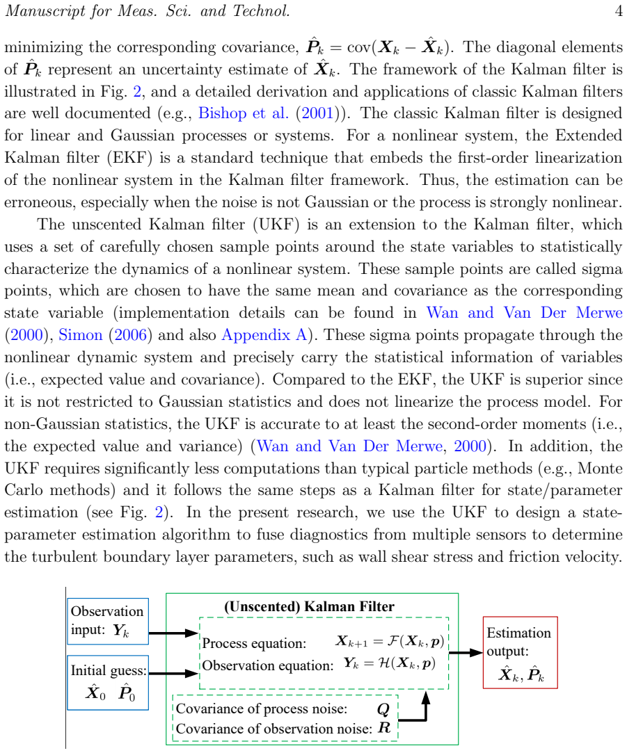
The load-bearing object is the unscented Kalman filter (UKF) used as a parameter estimator, with an observation function $H$ that embeds the modified Musker profile $\tilde{u}(y) = u_\tau( u^+_{\mathrm{musker}} + u^+_{\mathrm{bump}})$ for $0 \le y \le \delta$, together with the Preston tube relation $\log_{10}(\tau_w D^2/\rho\nu^2) = K_1 \log_{10}(\Delta P D^2/\rho\nu^2) - K_2$, the direct shear-stress relation $\tau_w = \rho u_\tau^2$, a soft no-slip condition, and the boundary-layer-thickness and freestream-velocity observations. The UKF propagates $2L+1$ $\sigma$ points through this nonlinear map, so the posterior mean and covariance of the state vector $X = [\tau_w, u_\tau, \delta, \Pi, U_\infty]$ are computed without linearizing $H$. The observation covariance $R$ carries the measurement uncertainties—including the banded, correlated PIV uncertainty from overlapped interrogation windows—and the process covariance $Q$ encodes the assumed spread of the parameters themselves; the filter then recursively minimizes the estimation covariance, not a fitting error norm, which is how it produces both estimates and their uncertainties.

What would settle it

Run the same UKF on a turbulent boundary layer with a known, independently measured friction velocity (for example, a DNS with an adverse or favorable pressure gradient, or a well-characterized experiment with $\beta$ of order $\pm 0.5$), without changing the embedded Musker profile; if the posterior 95% intervals fail to cover the true $u_\tau$, that failure pinpoints the profile model as the limiting assumption. A softer test: in the current experimental setup, hold the PIV data fixed and deliberately mis-enter the Preston tube calibration constants $K_1, K_2$; if the UKF estimate of $\tau_w$ shifts by an amount larger than its output covariance, the filter's uncertainty quantification is underweighting a known systematic source.

Watch

Extended reading notes

Core claim

On its own terms, the paper's central claim is that a UKF-based data assimilation scheme, with the observation function built from the modified Musker velocity profile, the Preston-tube calibration, the direct wall-shear relation $\tau_w = \rho u_\tau^2$, and the no-slip/edge boundary conditions, can fuse stereoscopic PIV, Preston tube, and MEMS shear-sensor data into accurate estimates of $u_\tau$ and $\tau_w$ with quantified uncertainty. In DNS-based synthetic tests the relative errors are below about 1% for $u_\tau$ and 2% for $\tau_w$ across a wide range of PIV resolutions and wall offsets, and the estimates carry a covariance that is statistically consistent with the true values. In the experimental application the UKF yields $u_\tau = 4.23 \pm 0.02$ m/s and $\tau_w = 20.73 \pm 0.21$ Pa, consistent with Preston tube, Clauser-chart, and control-volume values, while the MEMS sensor sits outside this range and is treated as biased. The paper frames the contribution as a general framework: replace the embedded flow-profile model and the sensor equations, and the same filtering machinery applies to other boundary-layer flows and measurement combinations.

Load-bearing premise

The entire observation model assumes that the mean velocity profile of the flow is exactly described by the modified Musker profile, which is a zero-pressure-gradient model; the experimental flow has a measurable favorable pressure gradient (β = −0.029), and the paper notes that pressure-gradient cases would need a different profile.

Editorial extensions

If this is right

Wall-shear estimation becomes a single, statistically principled fusion step rather than a choice among disagreeing techniques.
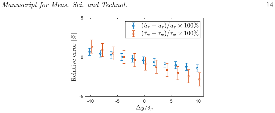
The framework's robustness to wall-position error (less than 0.5% shift in $\tau_w$ over ±10 viscous wall units) relaxes the near-wall alignment requirements of PIV.
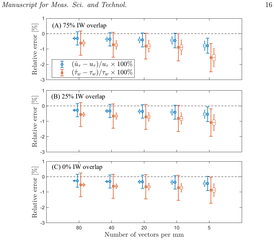
Even very coarse PIV data (about 8 usable vectors in the profile) suffices for roughly 0.5% accuracy in $u_\tau$ and 1% in $\tau_w$, so the method is applicable where near-wall optical access is limited.
The same filter structure can be re-run with a different embedded profile model to extend to pressure-gradient boundary layers, as the authors themselves suggest.
Because the filter outputs a covariance, its estimates can be merged or compared with other uncertainties (e.g., control-volume drag) in subsequent analyses.

Reading between the lines

Editorial extensions of the paper, not claims the author makes directly.

A natural extension the authors leave implicit: use the output covariance as a diagnostic to detect model bias—if the UKF's 2σ bands and independent measurements (like LISF) systematically disagree, the embedded profile, not the sensors, is the suspect.
The Monte Carlo calibration checks for PIV resolution suggest a testable prescription for PIV processing: reduce interrogation-window overlap when resolution is low, because correlated uncertainty degrades the filter more than uncorrelated noise.
One could generalize the state vector to include a pressure-gradient parameter or wall-roughness height, letting the UKF estimate them along with $u_\tau$, provided the observation model is extended accordingly.

Share X Bluesky LinkedIn Reddit HN

Signed reviews

No signed human review yet.

Editorial analysis

A structured set of objections, weighed in public.

Desk editor's note, referee report, and a circularity audit.

Desk Editor's Note

read the letter

Two things worth knowing. First, this is a genuinely useful application paper: a UKF that fuses SPIV, Preston tube, and MEMS shear data to estimate u_tau and tau_w, with correlated PIV covariances handled properly. Second, the headline claim—"quantified uncertainty"—does not hold up for the experimental case, because the observation model treats the modified Musker profile as exact and the independent LISF check is outside the reported interval. That is a real problem, not a nitpick.

What's new is the specific process/observation model and the way the authors build R with off-diagonal PIV covariance. The UKF itself is textbook, but the assembly is new and practical. The validation is thorough: 5,000 Monte Carlo runs, wall-offset sweeps, resolution and overlap sweeps. The DNS database is open access, which is real credit. The paper is also honest about the zero-pressure-gradient limitation in Section 6.

Where it's soft. The model-form error in Musker is not in the UKF covariance. The experimental flow has beta = -0.029; the paper says a different profile is needed for pressure gradients, yet applies the ZPG model to this flow. The result: UKF gives tau_w = 20.73 +/- 0.21 Pa, while LISF gives 17.3 [15.5, 18.3] Pa. The 2-sigma intervals don't overlap. The paper attributes this to Mach number differences, but the magnitude suggests unmodeled bias. Because the filter has no model-error term, adding more PIV data will tighten the covariance around whatever bias Musker has. So the uncertainty is understated. Also, the abstract says "turbulent boundary layer" for the DNS while the full text says "channel flow"—should be corrected. The synthetic Preston data is generated with the same Ferriss correlation used in the estimator, so that part of the validation tests noise robustness, not model correctness.

Minor: no code or processed data released, which hurts reproducibility. The experimental cross-checks with control volume and Clauser all agree with the UKF around 20-21 Pa, so I'm not arguing the bias is definitely in the UKF; the point is the reported covariance overstates what is known.

Who benefits: experimental groups working on skin-friction metrology and multi-sensor fusion. Worth a serious referee; it should go to review with a major-revision expectation. The method is well-built and reproducible, but the uncertainty claim needs either model-error handling or a scaled-back statement.

Referee Report

3 major / 4 minor

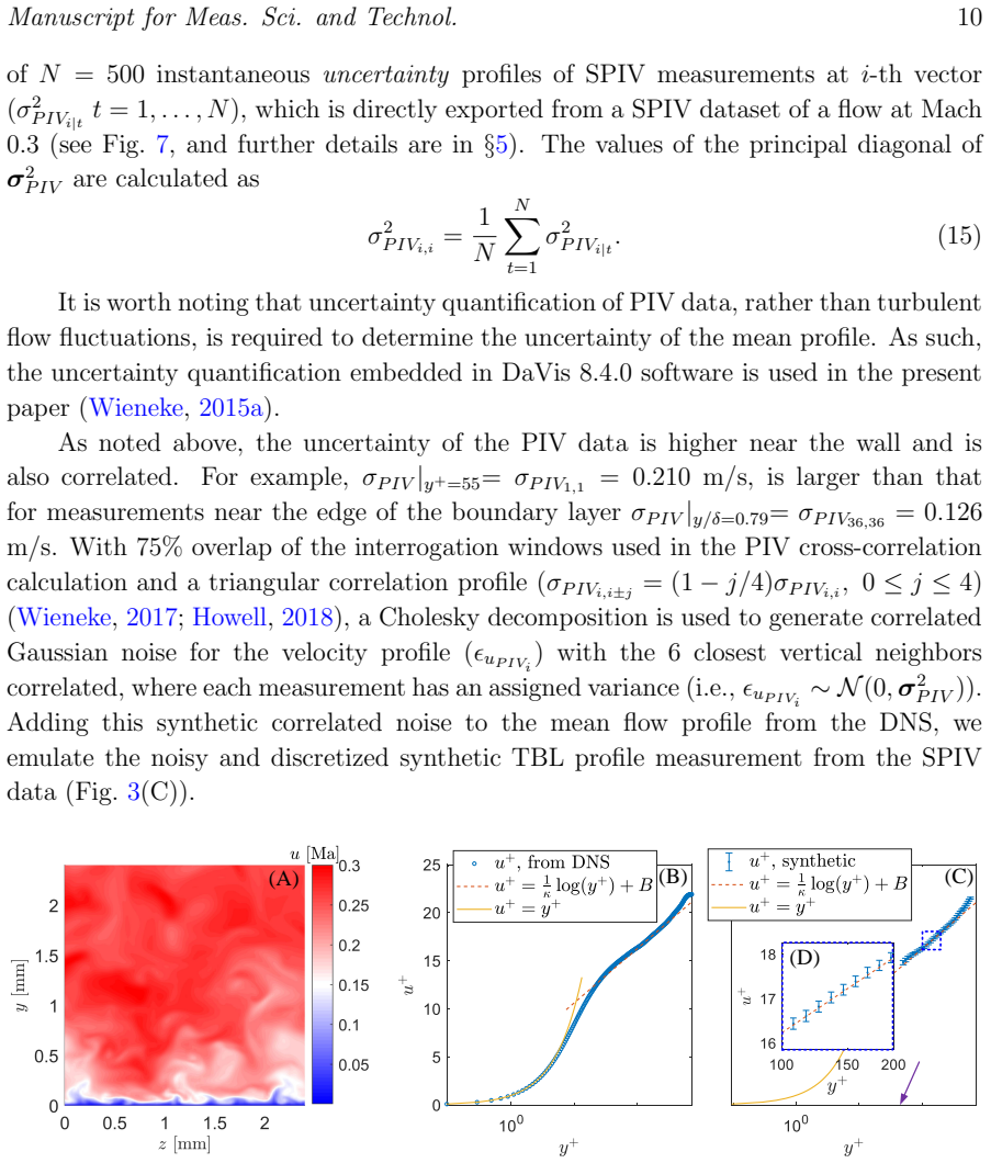
Summary. This paper presents a UKF-based data assimilation framework for estimating turbulent boundary layer parameters (friction velocity u_tau, wall shear stress tau_w, boundary layer thickness delta, wake parameter Pi, and freestream velocity U_infinity) by fusing Stereo-PIV velocity profiles, Preston tube differential pressure, a MEMS shear-stress sensor, and boundary-condition pseudo-measurements. The observation model combines a modified Musker mean-velocity profile, the Ferriss/Head-Rechenberg Preston calibration, and a direct shear-stress relation; the process model enforces physical relationships among the state variables. The framework is validated on synthetic noisy data constructed from a Mach 0.3 channel DNS, including 5,000-run Monte Carlo tests with wall-offset, resolution, and interrogation-window-overlap sweeps, and is then applied to Mach 0.3 wind-tunnel data, with control-volume analysis and LISF used as independent cross-checks. The paper claims that the algorithm is robust to uncertain and gappy experimental data and provides accurate estimates with quantified uncertainty.

Significance. The framework is potentially useful because it offers a principled way to fuse heterogeneous wall-shear diagnostics while propagating correlated and gappy PIV uncertainties into the final estimate; the Monte Carlo validation is thorough, and the open-access DNS database is a practical strength. The treatment of correlated PIV uncertainty in the observation covariance R is a genuine contribution. However, the central claim of quantified uncertainty is only as strong as the observation model, and the experimental application uses a zero-pressure-gradient profile in a flow with a measured nonzero pressure-gradient parameter (beta = -0.029) while the independent LISF result lies far outside the reported posterior interval. These issues must be resolved before the uncertainty-quantification claim is supportable.

major comments (3)

[§5, Table 1, §6; Eq. (8), Eq. (10)] The experimental flow has a measured favorable pressure gradient (beta = -0.029 in Table 1), yet the observation function H in Eq. (8) embeds the modified Musker profile of Eq. (1), a zero-pressure-gradient model. Section 6 concedes that pressure-gradient cases require a different flow-profile model, but no model-form error is added to the observation covariance R in Eq. (10). As a result, the posterior covariance reported in Table 2 does not represent structural bias in the velocity-profile model. The discrepancy with the independent LISF measurement (UKF tau_w = 20.73 ± 0.21 Pa vs. LISF 17.3 [15.5, 18.3] Pa) is a concrete symptom: even the 2σ UKF interval is disjoint from the LISF 95% interval, and the Mach-number/LISF-uncertainty explanation in Section 5 does not quantitatively account for a roughly 17% offset. The authors should either re-estimate with a pressure-gradient-aware profile, add an explicit model-error covariance to R, or validate on a case with negligible pressure gradient, and should temper the uncertainty claim accordingly.
[§4, Eq. (2), Eq. (8)] The synthetic validation is self-consistent with respect to the empirical correlations that the estimator inverts. The synthetic Preston pressure is generated by applying the Ferriss/Head-Rechenberg relation (Eq. 2) to the DNS velocity at y+ ≈ 46, and the velocity observations are generated from a DNS profile that is then inverted through the same modified Musker model used in H. Thus the 5,000-run Monte Carlo tests characterize robustness to noise, wall offset, resolution, and overlap, but they cannot detect bias in the Musker profile or the Preston calibration. The experimental LISF comparison in Table 2 is the only test that can expose such bias, and it does. This limitation should be stated explicitly, and the validation section should not be read as evidence that model-form error is negligible.
[§3 and §4, Eqs. (8), (10); text near Eq. (5)] The no-slip pseudo-measurement is specified inconsistently with the embedded model. The text states that the modified Musker profile gives u+(y+ = 0) = -0.0087, and the pseudo-measurement uncertainty is set to sigma_0 = 10^-3 u_tau in §4. The known model discrepancy at the wall is therefore about 8.7 sigma_0, yet the pseudo-measurement is treated as a zero-mean observation. This understates the uncertainty of the no-slip constraint, biases the posterior slightly, and artificially shrinks the covariance. The authors should set sigma_0 at least comparable to |u+(0)| u_tau or include the known wall discrepancy as a bias term.

minor comments (4)

[§3, after Eq. (8)] The text reads 'Masker's profile' where 'Musker's profile' is intended; please correct the typo.
[§4, Eq. (15)] The sentence introducing Eq. (15) mixes the covariance matrix sigma_PIV with its diagonal entries; clarify that Eq. (15) defines the diagonal elements of the covariance matrix.
[§4, Q specification] The process noise covariance Q is chosen heuristically from 'significant digits' of the state variables, and no sensitivity study is reported. Given the paper's emphasis on quantified uncertainty, a short sensitivity test varying Q over an order of magnitude would strengthen the claim.
[Figure 6 and surrounding text] The statement that '8 vectors (corresponding to 5 vectors/mm)' is ambiguous; please state explicitly the number of PIV samples and the physical resolution for each tested case.

Circularity Check

0 steps flagged · score 0.0 of 10

No significant circularity: the UKF estimation fuses independent measurements and is cross-validated externally.

full rationale

The UKF estimator inverts three independent measurement models (modified Musker profile h1, Preston correlation h2, and the shear-stress relation h3) for unknown TBL parameters. The estimates are not equal to any input by construction: the state-vector entries tau_w, u_tau, delta, Pi, and U_infinity are not defined in terms of the observations except through physical measurement equations. The DNS validation is not circular because the synthetic SPIV profiles come from a DNS channel flow (u_tau = 4.784 m/s), not from the Musker profile, and the synthetic Preston pressure is obtained from the DNS velocity at y+ = 46 rather than from the same Ferriss correlation; the paper even reports that the synthetic Preston tube gives a tau_w about 7% lower than the DNS value, so the observation model is tested against a mismatched truth. The experimental application fuses SPIV, Preston, and MEMS data with independently reported sensor uncertainties and cross-validates against control-volume and LISF measurements; no fitted parameter is renamed as a prediction. Section 6's caveat that the modified Musker profile is for zero-pressure-gradient flows and that pressure-gradient cases require a different profile is a model-form limitation relevant to uncertainty calibration, not a self-referential reduction; omitting that model error from the UKF covariance is a correctness risk but not circularity. The only self-citations (the open-access DNS database and the control-volume details in Gustavsson et al.) are not load-bearing for the central estimation claim.

Assumptions & free parameters 4 free parameters · 6 assumptions · 0 invented entities

The central claim relies on semi-empirical mean-velocity and Preston-tube models from prior literature, on the unscented transform approximation, and on hand-set filter covariances Q and sigma_0. No new entities are introduced. Model-form error is the main unquantified risk, visible in the LISF disagreement.

free parameters (4)

Process noise covariance Q = diag(10^-4, 10^-4, 4e-8, 10^-4, 10^-2)
Chosen by hand as order-of-magnitude estimates of state precision (Section 4). Affects filter gain and reported uncertainty; no systematic sensitivity study is reported.
No-slip pseudo-measurement uncertainty sigma_0 = 10^-3 u_tau
Set as an order-of-magnitude estimate so the UKF softly enforces no-slip (Section 4).
Synthetic noise parameters (sigma_PT, sigma_SSS, sigma_delta, sigma_Uinf) = 0.01 DeltaP, tau_w/sqrt(3), 0.05 delta, 0.02 Uinf
Assumed in the synthetic validation to mimic experimental uncertainty; not tested for sensitivity.
UKF sigma-point parameters alpha, beta = 0.01, 2
Standard values from Wan and Van Der Merwe; alpha robustness tested over 10^-5 to 10^-1.

assumptions (6)

domain assumption Modified Musker profile (Eq. 1) accurately represents the mean velocity profile of the flow.
The observation function H embeds this semi-empirical ZPG model; any model bias directly biases the estimates and makes covariance overconfident. The paper notes in Section 6 that pressure-gradient cases need a different profile.
domain assumption Preston tube correlation (Eq. 2) with K1=0.889, K2=1.400 is valid in the tested regime.
Used to form observation h2; constants from Ferriss (1965), not re-derived here. The synthetic validation generates Preston data with the same correlation, so it does not test this assumption.
domain assumption Wake-parameter relation f2 (Eq. 13) with kappa=0.41, B=5.0 holds.
Adds a deterministic link between Pi, u_tau, delta, and U_infinity; if inaccurate, the filter is pulled toward wrong Pi and slightly wrong u_tau.
domain assumption The channel-flow DNS at Mach 0.3 is representative of a TBL for validation purposes.
Validation uses a channel flow, not a boundary layer (Section 4); the outer region and wake parameters differ, so the validation does not exercise the boundary-layer edge model realistically.
domain assumption Measurement noise covariances in R are correctly estimated from instruments.
PIV uncertainty from DaVis, Preston from transducer spec, MEMS from its datasheet; if these are miscalibrated, the fusion weights and output uncertainty are wrong.
standard math UKF framework assumptions: zero-mean noise with known covariance and second-order moment approximation.
Standard UKF mathematics from Wan and Van Der Merwe; not specific to the physics.

how reviews work

0 comments

Cite this review

Pith. "Pith review of Unscented Kalman filter (UKF) based nonlinear parameter estimation for a turbulent boundary layer: a data assimilation framework." pith.science (2026). https://pith.science/paper/53JVS47A

@misc{pith2026190807604,
  author       = {Pith},
  title        = {Pith review of: Unscented Kalman filter (UKF) based nonlinear parameter estimation for a turbulent boundary layer: a data assimilation framework},
  year         = {2026},
  howpublished = {\url{https://pith.science/paper/53JVS47A}},
  note         = {Machine review of arXiv:1908.07604}
}

abstract

A turbulent boundary layer is an essential flow case of fundamental and applied fluid mechanics. However, accurate measurements of turbulent boundary layer parameters (e.g., friction velocity $u_\tau$ and wall shear $\tau_w$), are challenging, especially for high speed flows (Smits et al., 2011). Many direct and/or indirect diagnostic techniques have been developed to measure wall shear stress (Vinuesa et al., 2017). However, based on different principles, these techniques usually give different results with different uncertainties. The current study introduces a nonlinear data assimilation framework based on the Unscented Kalman Filter that can fuse information from i) noisy and gappy measurements from Stereo Particle Image Velocimetry, a Preston tube, and a MEMS shear stress sensor, as well as ii) the uncertainties of the measurements to estimate the parameters of a turbulent boundary layer. A direct numerical simulation of a fully developed turbulent boundary layer flow at Mach 0.3 is used first to validate the data assimilation algorithm. The algorithm is then applied to experimental data of a flow at Mach 0.3, which are obtained in a blowdown wind tunnel facility. The UKF-based data assimilation algorithm is robust to uncertain and gappy experimental data and is able to provide accurate estimates of turbulent boundary layer parameters.

Figures

Figures reproduced from arXiv: 1908.07604 by the authors.

**Figure 2.** Kalman filter framework for state and/or parameter estimation. A Kalman [PITH_FULL_IMAGE:figures/full_fig_p004_2.png] view at source ↗

**Figure 3.** DNS data and DNS-based synthetic data. (A) A slice of the instantaneous [PITH_FULL_IMAGE:figures/full_fig_p010_3.png] view at source ↗

Figures from the paper (7 more)

**Figure 4.** Figure 4: UKF estimation of TBL parameters. The black solid lines indicate the [PITH_FULL_IMAGE:figures/full_fig_p012_4.png]

**Figure 5.** Figure 5: Averaged relative error in the UKF-estimated wall shear stress and friction [PITH_FULL_IMAGE:figures/full_fig_p014_5.png]

**Figure 6.** Figure 6: Relative error in the UKF-estimated wall shear stress and friction velocity [PITH_FULL_IMAGE:figures/full_fig_p016_6.png]

**Figure 7.** Figure 7: Averaged streamwise velocity profile (A) and uncertainty (B) from [PITH_FULL_IMAGE:figures/full_fig_p017_7.png]

**Figure 8.** Figure 8: UKF estimation results with experimental measurements. The red dashed [PITH_FULL_IMAGE:figures/full_fig_p018_8.png]

**Figure 9.** Figure 9: Relative shift in the UKF-estimated wall shear stress and friction velocity, [PITH_FULL_IMAGE:figures/full_fig_p019_9.png]

**Figure 10.** Figure 10: Schematic of laser interferometer skin friction meter setup (A), and the [PITH_FULL_IMAGE:figures/full_fig_p019_10.png]

Discussion (0). Continue with ORCID to comment.

Reference graph

Works this paper leans on

5 extracted references · 4 canonical work pages

[1]

M., Nichols, J

Bermejo-Moreno, I., Bodart, J., Larsson, J., Barney, B. M., Nichols, J. W. and Jones, REFERENCES 25 S. (2013). Solving the compressible Navier-Stokes equations on up to 1.97 million cores and 4.1 trillion grid points, SC’13: Proceedings of the International Conference on High Performance Computing, Networking, Storage and Analysis , pp. 1–10. Bhattacharya...

work page 2013
[8]

A., Monkewitz, P

Chauhan, K. A., Monkewitz, P. A. and Nagib, H. M. (2009). Criteria for assessing experiments in zero pressure gradient boundary layers, Fluid Dynamics Research 41(2): 021404. Clauser, F. H. (1954). Turbulent boundary layers in adverse pressure gradients, Journal of the Aeronautical Sciences 21(2): 91–108. Clauser, F. H. (1956). The Turbulent Boundary Laye...

work page 2009
[41]

Cantwell, B. J. (2018). Fundamentals of Compressible Flow , Stanford University, chapter

work page 2018
[68]

and Grottadaurea, M

Rona, A. and Grottadaurea, M. (2010). Generalized coles’ law and outer layer conformal mapping, Journal of Hydraulic Research 48(5): 674–679. Sciacchitano, A., Neal, D. R., Smith, B. L., Warner, S. O., Vlachos, P. P., Wieneke, B. and Scarano, F. (2015). Collaborative framework for piv uncertainty quantiﬁcation: comparative assessment of methods, Measureme...

2010
[478]

Musker, A. (1979). Explicit expression for the smooth wall velocity distribution in a turbulent boundary layer, AIAA Journal 17(6): 655–657. Naughton, J. W. and Sheplak, M. (2002). Modern developments in shear-stress measurement, Progress in Aerospace Sciences 38(6-7): 515–570. ¨Orl¨ u, R., Fransson, J. H. and Alfredsson, P. H. (2010). On near wall measur...

work page 1979

Pith tools

Reviewed August 14, 2026 · model on record in the stance chip above.

[1] [1]

M., Nichols, J

Bermejo-Moreno, I., Bodart, J., Larsson, J., Barney, B. M., Nichols, J. W. and Jones, REFERENCES 25 S. (2013). Solving the compressible Navier-Stokes equations on up to 1.97 million cores and 4.1 trillion grid points, SC’13: Proceedings of the International Conference on High Performance Computing, Networking, Storage and Analysis , pp. 1–10. Bhattacharya...

work page 2013

[2] [8]

A., Monkewitz, P

Chauhan, K. A., Monkewitz, P. A. and Nagib, H. M. (2009). Criteria for assessing experiments in zero pressure gradient boundary layers, Fluid Dynamics Research 41(2): 021404. Clauser, F. H. (1954). Turbulent boundary layers in adverse pressure gradients, Journal of the Aeronautical Sciences 21(2): 91–108. Clauser, F. H. (1956). The Turbulent Boundary Laye...

work page 2009

[3] [41]

Cantwell, B. J. (2018). Fundamentals of Compressible Flow , Stanford University, chapter

work page 2018

[4] [68]

and Grottadaurea, M

Rona, A. and Grottadaurea, M. (2010). Generalized coles’ law and outer layer conformal mapping, Journal of Hydraulic Research 48(5): 674–679. Sciacchitano, A., Neal, D. R., Smith, B. L., Warner, S. O., Vlachos, P. P., Wieneke, B. and Scarano, F. (2015). Collaborative framework for piv uncertainty quantiﬁcation: comparative assessment of methods, Measureme...

2010

[5] [478]

Musker, A. (1979). Explicit expression for the smooth wall velocity distribution in a turbulent boundary layer, AIAA Journal 17(6): 655–657. Naughton, J. W. and Sheplak, M. (2002). Modern developments in shear-stress measurement, Progress in Aerospace Sciences 38(6-7): 515–570. ¨Orl¨ u, R., Fransson, J. H. and Alfredsson, P. H. (2010). On near wall measur...

work page 1979