REVIEW 3 major objections 6 minor 29 references
Risk-Efficient Bayesian Data Synthesis for Privacy Protection
T0 review · 3 major / 6 minor · reviewed 2026-08-14 · deepseek-v4-flash
Pith's one-line read Record-level risk weights built from pairwise identification probabilities make synthetic data safer and more useful than marginal weighting.
desk verdict Useful risk-weighting framework for synthetic data, but the identification risk measure is miscalibrated under the paper's own intruder model, so the quantitative claims need rework. read the letter →
The pith
A machine-rendered reading of the paper's core claim, the machinery that carries it, and where it could break.
The reading
What carries the argument
The central object is the record-indexed pseudo-likelihood weight $\alpha_i \in [0,1]$, used as an exponent on each record's likelihood contribution in the pseudo posterior. The marginal form $\alpha_i = 1 - IR^c_i$ surgically downweights isolated high-risk records, while the pairwise form $\alpha^{\mathrm{pw}}_i = 1 - \frac{1}{|M_{p,i}|-1}\sum_{j\ne i} IR^c_{i,j}$ averages joint identification risks and thereby ties the downweighting of records together. The mechanism works by deliberately misspecifying the likelihood in high-risk regions, pulling synthetic values for those records toward the main modes while preserving the rest of the distribution. The pair dependence is what prevents the marginal approach's whack-a-mole failure, because shrinking one record no longer leaves its moderate-risk neighbours uncovered.
What would settle it
A concrete falsifier is an intruder simulation that matches released synthetic records using richer information, such as additional covariates or a different closeness radius, and compares the success rate with the paper's predicted $IR_i$ values. If the simulation succeeds materially more often than the predicted risks on the same released datasets, the weight construction is not protecting against the threat it purports to measure.
Extended reading notes
Core claim
The central claim is that record-indexed risk weights applied as likelihood exponents convert a Bayesian synthesizer into a privacy-adjusted synthesizer. The disclosure risk of record $i$ is defined as the fraction of same-pattern records whose synthetic values lie outside a ball of radius $r$ around the true value $y_i$, multiplied by an indicator that record $i$'s own synthetic value is close; the confidential-data version $IR^c_i$ sets $\alpha_i = 1 - IR^c_i$. The pseudo posterior $p_{\alpha}(\theta \mid y, X, \eta) \propto \prod_i p(y_i \mid X,\theta)^{\alpha_i}\,p(\theta \mid \eta)$ deliberately downweights high-risk contributions. The pairwise extension replaces the marginal risk with an average over joint pairwise risks, $\alpha^{\mathrm{pw}}_i = 1 - \frac{1}{|M_{p,i}|-1}\sum_{j\ne i} IR^c_{i,j}$, which makes the weights dependent within each pattern. In the consumer-expenditure application the pairwise synthesizer is claimed to compress the by-record risk distribution, reduce the maximum risks, and preserve utility much better than the marginal synthesizer at about the same mean risk.
Load-bearing premise
The load-bearing premise is that an intruder knows each record's true income and the pattern variables, and judges closeness using the agency-chosen radius $r$; if an actual intruder has more information, uses a different closeness rule, or targets records in another way, the weights downweight the wrong records and the reported risk profiles are not true disclosure risk.
Editorial extensions
If this is right
- A statistical agency can take any existing Bayesian synthesizer and tune its privacy by exponentiating likelihood contributions with the record-specific weights, without redesigning the model.
- Marginal weighting lowers the overall risk distribution but can raise risk for moderate-risk records, so agencies should examine record-level risk profiles rather than only averages before release.
- Pairwise weighting mitigates the whack-a-mole problem and gives a more compressed, better-controlled risk distribution at about the same mean risk, with utility close to the unweighted synthesizer.
- Risk-weighted synthesis protects high-risk records throughout the income distribution, unlike topcoding, which leaves many high-risk non-tail records untouched.
- A scaling constant and an additive shift on the weights provide local controls for trading a little more risk for more utility, letting agencies tune the release to their policy target.
Reading between the lines
- If the pairwise construction is applied to multivariate synthesis, the ball $B(y_i,r)$ becomes a multidimensional region and the same joint-coverage logic would require a closeness definition for mixed categorical and continuous variables; this is a natural extension the paper leaves open.
- Because the weights are plug-in estimates from one confidential dataset, the method's risk guarantee is conditional on those estimates; agencies could quantify the added uncertainty by bootstrapping the risk estimation step.
- A useful benchmark would compare this intruder-model approach with a formally private baseline at matched levels of worst-case record risk; the paper contrasts with such guarantees conceptually but does not run the comparison.
Signed reviews
Editorial analysis
A structured set of objections, weighed in public.
Referee Report
Summary. The paper proposes a general framework for inducing privacy protection into any Bayesian synthesizer by exponentiating each likelihood contribution by a record-indexed weight in [0,1] that is inversely proportional to an estimated identification risk. The marginal version computes a risk IR^c_i for each confidential record, sets the weight to 1-IR^c_i, and draws synthetic data from the resulting pseudo posterior. Applied to 2017 Q1 Consumer Expenditure Survey family income, it reports lower risk than unweighted synthesis, but also reduced utility and a "whack-a-mole" effect whereby some moderate-risk records become more identifiable. A pairwise version constructs weights from joint risks for pairs of records in the same pattern and is reported to mitigate the whack-a-mole effect and improve utility. A simulation with negative binomial mixtures and sensitivity analyses for the radius r and the number of released datasets L support the qualitative conclusions.
Significance. The framework is potentially valuable for statistical agencies: it is synthesizer-agnostic, targets risky records rather than applying a blunt global transformation like topcoding, and introduces a concrete diagnosis (whack-a-mole) plus a pairwise dependence mechanism that produces more compressed risk profiles. The CE application is realistic, the source code is available, and the sensitivity analyses for r and L are useful. However, the central risk metric is mislabeled and internally inconsistent with the stated intruder model, and the CE application leaves an unresolved ambiguity about how the logarithmic transformation handles negative income values. These issues must be resolved before the claimed privacy guarantees can be accepted.
major comments (3)
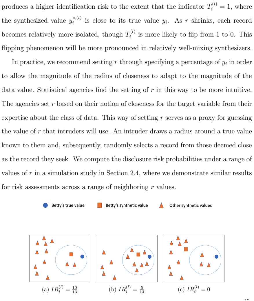
- [Section 2.1, Eq. (1)] The quantity in Eq. (1) is not the probability of identification under the intruder model described in Section 2.1. The text states that the intruder randomly selects a record among those whose synthetic values lie in B(y_i,r). If T_i^(l)=1 and C equals the number of records in the pattern with synthetic values in B(y_i,r), the probability of correctly identifying record i is 1/C, not (|M|-C)/|M| times T_i. Eq. (1) equals (|M|-C)/|M| when T_i=1. The two quantities rank records differently: for C=1 and |M|=10, Eq. (1) gives 0.9 while the actual probability is 1; for C=2 and |M|=100, Eq. (1) gives 0.98 while the actual probability is 0.5. Since Eq. (3) defines the weights as 1-IR^c_i on the same quantity, the weights can downweight a less identifiable record more heavily than a uniquely identifiable one. All reported risk reductions in Sections 2.3, 2.4, and 3.2 and Tables 2-3 and Figures 2, 3, 8, and 9 are expressed in units of this index, so the central claim about lower identification risk is not established as a claim about probability of identification. Please either correct Eq. (1) to match the stated intruder model or explicitly redefine IR as a coverage/rareness index that is not a probability of identification, and adjust the interpretation of the weights and risk profiles accordingly.
- [Section 3.1, Eq. (6)] The definition of the pairwise risk event is inconsistent. The prose says the probability is computed for h lying in the intersection y_h in B(y_i,r) and y_h in B(y_j,r), but the formula counts h with y_h not in B(y_i,r) and y_h not in B(y_j,r), i.e., outside both balls. The complement of the intersection of the two balls is "outside at least one ball," not "outside both." The Supplementary Material Algorithm 1 repeats this issue and also uses B(y_j,r) in both clauses. Because alpha_{i,j}=1-IR^c_{i,j} and the normalized weights in Eqs. (8)-(9) depend on these pairwise probabilities, the pairwise synthesizer needs a corrected, unambiguous formula.
- [Section 2 and Table 1] Section 2 defines y_i as the logarithm of family income, while Table 1 reports family income in dollars and states that negative family income values occur (approximate range starting at -7K). The paper does not state how the logarithmic transformation handles nonpositive incomes, nor how the radius r = 20% of y_i is defined when y_i is negative. Since Eqs. (1)-(3) and the CE application depend on the ball B(y_i,r), this ambiguity affects the risk computations and weights for records with nonpositive income. Please state the transformation used (for example, adding a constant) or explicitly exclude nonpositive records and justify that restriction.
minor comments (6)
- [Abstract and Section 1] If the authors adopt the redefinition suggested in the first major comment, the phrase "probability of identification" should be changed to "identification risk index" or a similar term throughout the manuscript.
- [Figure 5b] The panel label "Whack-a-model" should read "Whack-a-mole."
- [Sections 2.3 and 3.2] Utility comparisons include bootstrapped confidence intervals, but the risk summaries in Figures 2 and 8 are point estimates only; reporting Monte Carlo uncertainty across the L=20 synthetic datasets (for example, for the mean and IQR of the risk distribution) would strengthen the risk comparisons.
- [Table 4] The four sub-tables in Table 4 share row labels Data, Synthesizer, and Marginal with no separate panel headings; consider adding clearer panel labels and units for the point estimates.
- [Section 2] The finite mixture synthesizer is deferred entirely to the Supplementary Material; a brief one-sentence description in the main text would help readers understand the likelihood that is being exponentiated.
- [Supplementary Material, Algorithm 1] Steps 2 and 3 contain typographical repetitions of B(y_j,r); these should be corrected to B(y_i,r) and B(y_j,r) respectively.
Circularity Check
No significant circularity: the risk metric is used both to set weights and to evaluate, but the reduction is empirical, and the paper's own whack-a-mole results show it is not forced by construction.
full rationale
The claimed derivation is not circular. The weights alpha_i^m = 1 - IR^c_i (Eq. 3) are a deterministic transform of the confidential-data risk index (Eq. 2), and the synthetic-data risk index (Eq. 1) is the same functional with the same radius r and the same patterns. This reuse is a limitation: the reported risk reductions are expressed in the units of the very quantity used to set the weights, so the CE risk comparisons are not an external validation of the risk model. It is not, however, circular in the derivation sense, because the synthetic risk IR_i is not a fitted parameter and is not algebraically equal to 1 - alpha_i. The paper's own whack-a-mole results (Fig. 3 and Fig. 5b) show records whose synthetic risk increases from the Synthesizer to the Marginal, which would be impossible if the reduction were forced by construction. Utility comparisons (Tables 4, 5, 7), the topcoding critique (Table 3), and the whack-a-mole observation are independent of the weighting identity. The only self-citations (Savitsky and Toth 2016; Williams and Savitsky 2018; Hu 2019) are background or analogy and are not load-bearing; no uniqueness theorem or ansatz is imported from them. The Section 1 caveat that intruder behavior assumptions 'could be unverifiable, in practice' is an acknowledged limitation, not a circular step. The skeptic's point that Eq. (1) miscalibrates the probability of identification under the paper's own intruder story is a correctness concern, not a circularity concern, and does not change this verdict.
Assumptions & free parameters
free parameters (4)
- radius r for closeness balls =
20% of y_i in CE; 15-30% explored in simulation
- L, number of released synthetic datasets =
20
- simulation mixture parameters (theta1, mu1, mu2, phi1, phi2) =
0.7, 100, 100, 20, 5
- supplementary tuning constants c and g =
c=1.5 and g=0.1 explored
assumptions (5)
- domain assumption Intruder model: the intruder knows true y_i, knows the pattern variables, and randomly selects among same-pattern records whose synthetic values are within B(y_i,r).
- domain assumption r = 20% of y_i is a valid notion of closeness for CE family income.
- standard math Exponentiating likelihood contributions by weights alpha_i yields a coherent pseudo posterior.
- domain assumption The truncated Dirichlet process finite mixture synthesizer adequately captures the confidential CE distribution.
- domain assumption All known-intruder patterns have at least two records.
Cite this review
Pith. "Pith review of Risk-Efficient Bayesian Data Synthesis for Privacy Protection." pith.science (2026). https://pith.science/paper/W5ITK6TK
@misc{pith2026190807639,
  author       = {Pith},
  title        = {Pith review of: Risk-Efficient Bayesian Data Synthesis for Privacy Protection},
  year         = {2026},
  howpublished = {\url{https://pith.science/paper/W5ITK6TK}},
  note         = {Machine review of arXiv:1908.07639}
}
read the original abstract
Statistical agencies utilize models to synthesize respondent-level data for release to the public for privacy protection. In this work, we efficiently induce privacy protection into any Bayesian synthesis model by employing a pseudo likelihood that exponentiates each likelihood contribution by an observation record-indexed weight in [0, 1], defined to be inversely proportional to the identification risk for that record. We start with the marginal probability of identification risk for a record, which is composed as the probability that the identity of the record may be disclosed. Our application to the Consumer Expenditure Surveys (CE) of the U.S. Bureau of Labor Statistics demonstrates that the marginally risk-adjusted synthesizer provides an overall improved privacy protection; however, the identification risks actually increase for some moderate-risk records after risk-adjusted pseudo posterior estimation synthesis due to increased isolation after weighting; a phenomenon we label "whack-a-mole". We proceed to construct a weight for each record from a collection of pairwise identification risk probabilities with other records, where each pairwise probability measures the joint probability of re-identification of the pair of records, which mitigates the whack-a-mole issue and produces a more efficient set of synthetic data with lower risk and higher utility for the CE data.
Figures


Figures from the paper (14 more)



Reference graph
Works this paper leans on
-
[1]
An, D. and Little, R. J. A. (2007) Multiple imputation: an alternative to top coding for statistical disclosure control. Journal of the Royal Statistical Society, Series A, 170, 923--940
work page 2007
-
[2]
Dimitrakakis, C., Nelson, B., Zhang, Z., Mitrokotsa, A. and Rubinstein, B. I. P. (2017) Differential privacy for bayesian inference through posterior sampling. J. Mach. Learn. Res., 18, 343--381
work page 2017
-
[3]
(2011) Synthetic Datasets for Statistical Disclosure Control
Drechsler, J. (2011) Synthetic Datasets for Statistical Disclosure Control. Springer: New York
work page 2011
-
[4]
Drechsler, J., Dundler, A., Bender, S., Rassler, S. and Zwick, T. (2008) A new approach for disclosure control in the iab establishment panel - multiple imputation for a better data access. Advances in Statistical Analysis, 439--458
work page 2008
- [5]
-
[6]
Dwork, C., McSherry, F., Nissim, K. and Smith, A. (2006) Calibrating noise to sensitivity in private data analysis. In Proceedings of the Third Conference on Theory of Cryptography, TCC'06, 265--284
work page 2006
-
[7]
(2019) Bayesian estimation of attribute and identification midisclosure risks in synthetic data
Hu, J. (2019) Bayesian estimation of attribute and identification midisclosure risks in synthetic data. Transactions on Data Privacy, 12, 61--89
work page 2019
-
[8]
Hu, J., Reiter, J. P. and Wang, Q. (2018) Dirichlet process mixture models for modeling and generating synthetic versions of nested categorical data. Bayesian Analysis, 13, 183--200
work page 2018
Show all 29 references
-
[9]
S., Spicer, S
Hundepool, A., Domingo-Ferrer, J., Franconi, L., Giessing, S., Nordholt, E. S., Spicer, S. and de Wolf, P. (2012) Statistical Disclosure Control. Wiley
2012
-
[10]
F., Kohnen, C
Karr, A. F., Kohnen, C. N., Oganian, A., Reiter, J. P. and Sanil, A. P. (2006) A framework for evaluating the utility of data altered to protect confidentiality. The American Statistician, 60, 224--232
2006
-
[11]
K., Reiter, J
Kinney, S. K., Reiter, J. P., Reznek, A. P., Miranda, J., Jarmin, R. S. and Abowd, J. M. (2011) Towards unrestricted public use business microdata: The synthetic L ongitudinal B usiness D atabase. International Statistical Review, 79, 363--384
2011
-
[12]
Little, R. J. A. (1993) Statistical analysis of masked data. Journal of Official Statistics, 9, 407--426
1993
-
[13]
and Hu, J
Manrique-Vallier, D. and Hu, J. (2018) Bayesian non-parametric generation of fully synthetic multivariate categorical data in the presence of structural zeros. Journal of the Royal Statistical Society, Series A, 181, 635--647
2018
-
[14]
Quick, H., Holan, S. H. and Wikle, C. K. (2018) Generating partially synthetic geocoded public use data with decreased disclosure risk using differential smoothing. Journal of the Royal Statistical Society, Series A, 181, 649--661
2018
-
[15]
Reiter, J. P. and Mitra, R. (2009) Estimating risks of identification disclosure in partially synthetic data. The Journal of Privacy and Confidentiality, 1, 99--110
2009
-
[16]
Rubin, D. B. (1993) Discussion statistical disclosure limitation. Journal of Official Statistics, 9, 461--468
1993
-
[17]
Savitsky , T. D. and Toth , D. (2016) Bayesian estimation under informative sampling . Electronic Journal of Statistics, 10, 1677--1708
2016
-
[18]
M., Nowok, B., Dibben, C
Snoke, J., Raab, G. M., Nowok, B., Dibben, C. and Slavkovic, A. (2018) General and specific utility measures for synthetic data. Journal of the Royal Statistical Society, Series A, 181, 663--688
2018
-
[19]
and Reiter, J
Wei, L. and Reiter, J. P. (2016) Releasing synthetic magnitude microdata constrained to fixed marginal totals. Statistical Journal of the IAOS, 32, 93--108
2016
-
[20]
Williams, M. R. and Savitsky, T. D. (2018) Bayesian pairwise estimation under dependent informative sampling. Electronic Journal of Statistics, 12, 1631--1661
2018
-
[21]
J., Reiter, J
Woo, M. J., Reiter, J. P., Oganian, A. and Karr, A. F. (2009) Global measures of data utility for microdata masked for disclosure limitation. The Journal of Privacy and Confidentiality, 1, 111--124
2009
-
[22]
Neal, R. M. (2000) Markov chain sampling methods for D irichlet process mixture models. Journal of Computational and Graphical Statistics, 9, 249--265
2000
-
[23]
Reiter, J. P. and Raghunathan, T. E. (2007) The multiple adaptations of multiple imputation. Journal of the American Statistical Association, 102, 1462--1471
2007
-
[24]
://mc-stan.org/
Stan Development Team (2016) RStan : the R interface to Stan . ://mc-stan.org/. R package version 2.14.1
2016
-
[25]
@esa ( ) , n @biblabelnum##1 ##1
\@ifclassloaded aguplus natbib The aguplus class already includes natbib coding, so you should not add it explicitly Type <Return> for now, but then later remove the command natbib from the document \@ifclassloaded nlinproc natbib The nlinproc class already includes natbib cod...
-
[26]
@stdbsttrue NAT@ctr \@lbibitem[ NAT@ctr ] \@lbibitem[#1]#2 \@ifundefined b@#2\@extra@b@citeb @num @parse #2 [ @natanchorstart #2 \@biblabel @num @natanchorend] @ifcmd#1()()\@nil #2 @lbibitem\@undefined @lbibitem\@lbibitem \@lbibitem[#1]#2 @lbibitem[#1] #2 @ @@label #2 @stdbst ...
-
[27]
@open @close @open @close and [1] URL: #1 \@ifundefined chapter * \@mkboth \@ifundefined NAT@sectionbib * \@mkboth * \@mkboth\@gobbletwo \@ifclassloaded amsart * \@ifclassloaded amsbook * \@ifundefined bib@heading @heading NAT@ctr thebibliography [1] @ \@biblabel NAT@ctr \@bib...
-
[28]
, " * write output.state after.block = add.period write newline
ENTRY address author booktitle chapter edition editor howpublished institution journal key month note number organization pages publisher school series title type url volume year label extra.label sort.label short.list INTEGERS output.state before.all mid.sentence after.senten...
-
[29]
write newline
" write newline "" before.all 'output.state := FUNCTION n.dashify 't := "" t empty not t #1 #1 substring "-" = t #1 #2 substring "--" = not "--" * t #2 global.max substring 't := t #1 #1 substring "-" = "-" * t #2 global.max substring 't := while if t #1 #1 substring * t #2 gl...
Reviewed August 14, 2026 · model on record in the stance chip above.
Discussion (0). Continue with ORCID to comment.